A Practical Guide for SQL Tuning
This guide is designed for TiDB SQL tuning beginners. It focuses on the following key principles:
- Low entry barrier: introducing tuning concepts and methods step by step.
- Practice-oriented: providing specific steps and examples for each optimization tip.
- Quick start: prioritizing the most common and effective optimization methods.
- Gentle learning curve: emphasizing practical techniques rather than complex theory.
- Scenario-based: using real-world business cases to demonstrate optimization effects.
Introduction to SQL tuning
SQL tuning is crucial for optimizing database performance. It involves systematically improving the efficiency of SQL queries through the following typical steps:
Identify high-impact SQL statements:
- Review the SQL execution history to find statements that consume significant system resources or contribute heavily to the application workload.
- Use monitoring tools and performance metrics to identify resource-intensive queries.
Analyze execution plans:
- Examine the execution plans generated by the query optimizer for the identified statements.
- Verify whether these plans are reasonably efficient and use appropriate indexes and join methods.
Implement optimizations:
Implement optimizations to inefficient SQL statements. Optimizations might include rewriting SQL statements, adding or modifying indexes, updating statistics, or adjusting database parameters.
Repeat these steps until:
- The system performance meets target requirements.
- No further improvements can be made to the remaining statements.
SQL tuning is an ongoing process. As your data volume grows and query patterns change, you should:
- Regularly monitor query performance.
- Re-evaluate your optimization strategies.
- Adapt your approach to address new performance challenges.
By consistently applying these practices, you can maintain optimal database performance over time.
Goals of SQL tuning
The primary goals of SQL tuning are the following:
- Reduce response time for end users.
- Minimize resource consumption during query execution.
To achieve these goals, you can use the following strategies.
Optimize query execution
SQL tuning focuses on finding more efficient ways to process the same workload without changing query functionality. You can optimize query execution as follows:
Improving execution plans:
- Analyze and modify query structures for more efficient processing.
- Use appropriate indexes to reduce data access and processing time.
- Enable TiFlash for analytical queries on large datasets and leverage the Massively Parallel Processing (MPP) engine for complex aggregations and joins.
Enhancing data access methods:
- Use covering indexes to satisfy queries directly from the index, avoiding full table scans.
- Implement partitioning strategies to limit data scans to relevant partitions.
Examples:
- Create indexes on frequently queried columns to significantly reduce resource usage, particularly for queries that access small portions of the table.
- Use index-only scans for queries that return a limited number of sorted results to avoid full table scans and sorting operations.
Balance workload distribution
In a distributed architecture like TiDB, balancing workloads across TiKV nodes is essential for optimal performance. To identify and resolve read and write hotspots, see Troubleshoot hotspot issues.
By implementing these strategies, you can ensure that your TiDB cluster efficiently utilizes all available resources and avoids bottlenecks caused by uneven workload distribution or serialization on individual TiKV nodes.
Identify high-load SQL
The most efficient way to identify resource-intensive SQL statements is by using TiDB Dashboard. You can also use other tools, such as views and logs, to identify high-load SQL statements.
Monitor SQL statements using TiDB Dashboard
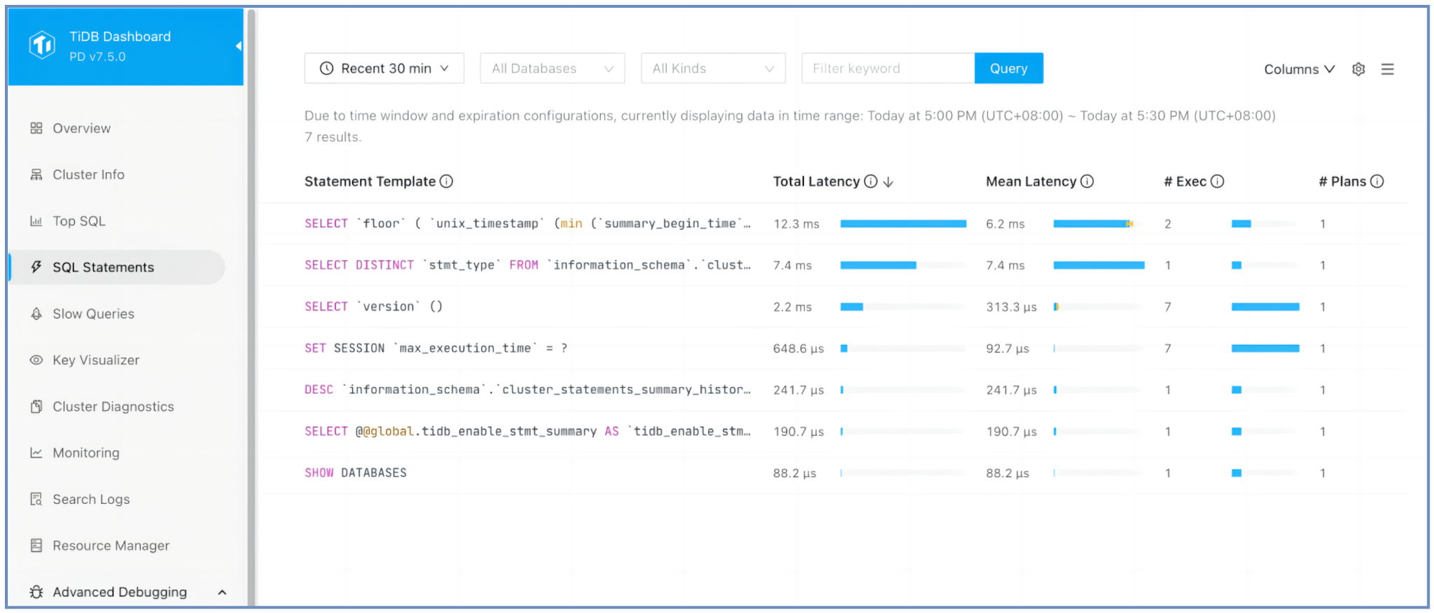
SQL Statements page
In TiDB Dashboard, navigate to the SQL Statements page to identify the following:
- The SQL statement with the highest total latency, which is the statement that takes the longest time to execute across multiple executions.
- The number of times each SQL statement has been executed, which helps identify statements with the highest execution frequency.
- Execution details of each SQL statement by clicking it to view
EXPLAIN ANALYZEresults.
TiDB normalizes SQL statements into templates by replacing literals and bind variables with ?. This normalization and sorting process helps you quickly identify the most resource-intensive queries that might require optimization.
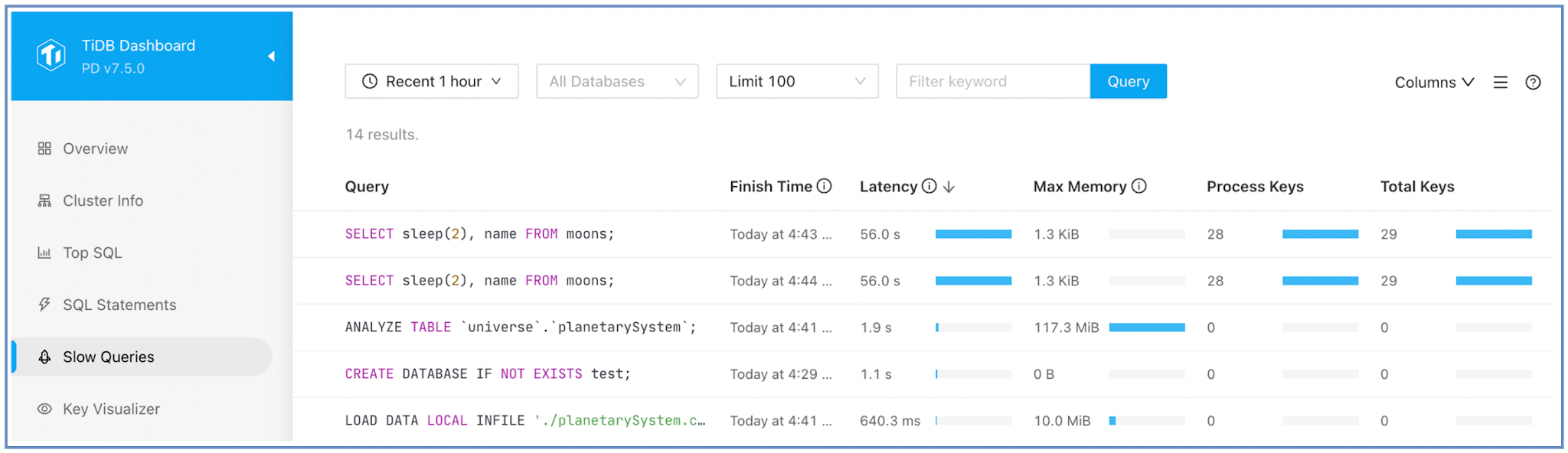
Slow Queries page
In TiDB Dashboard, navigate to the Slow Queries page to find the following:
- The slowest SQL queries.
- The SQL query that reads the most data from TiKV.
- The
EXPLAIN ANALYZEoutput by clicking a query for detailed execution analysis.
The Slow Queries page does not display SQL execution frequency. A query appears on this page if its execution time exceeds the tidb_slow_log_threshold configuration item for a single instance.
Use other tools to identify Top SQL
In addition to TiDB Dashboard, you can use other tools to identify resource-intensive SQL queries. Each tool offers unique insights and can be valuable for different analysis scenarios. Using a combination of these tools helps ensure comprehensive SQL performance monitoring and optimization.
- TiDB Dashboard Top SQL Page
- Logs: slow query log and expensive queries in TiDB log
- Views:
cluster_statements_summaryview andcluster_processlistview
Gather data on identified SQL statements
For the top SQL statements identified, you can use PLAN REPLAYER to capture and save SQL execution information from a TiDB cluster. This tool helps recreate the execution environment for further analysis. To export SQL execution information, use the following syntax:
PLAN REPLAYER DUMP EXPLAIN [ANALYZE] [WITH STATS AS OF TIMESTAMP expression] sql-statement;
Use EXPLAIN ANALYZE whenever possible, as it provides both the execution plan and actual performance metrics for more accurate insights into query performance.
SQL tuning guide
This guide provides practical advice for beginners on optimizing SQL queries in TiDB. By following these best practices, you can improve query performance and streamline SQL tuning. This guide covers the following topics:
Understand query processing
This section introduces the query processing workflow, optimizer fundamentals, and statistics management.
Query processing workflow
When a client sends a SQL statement to TiDB, the statement passes through the protocol layer of the TiDB server. This layer manages the connection between the TiDB server and the client, receives SQL statements, and returns data to the client.
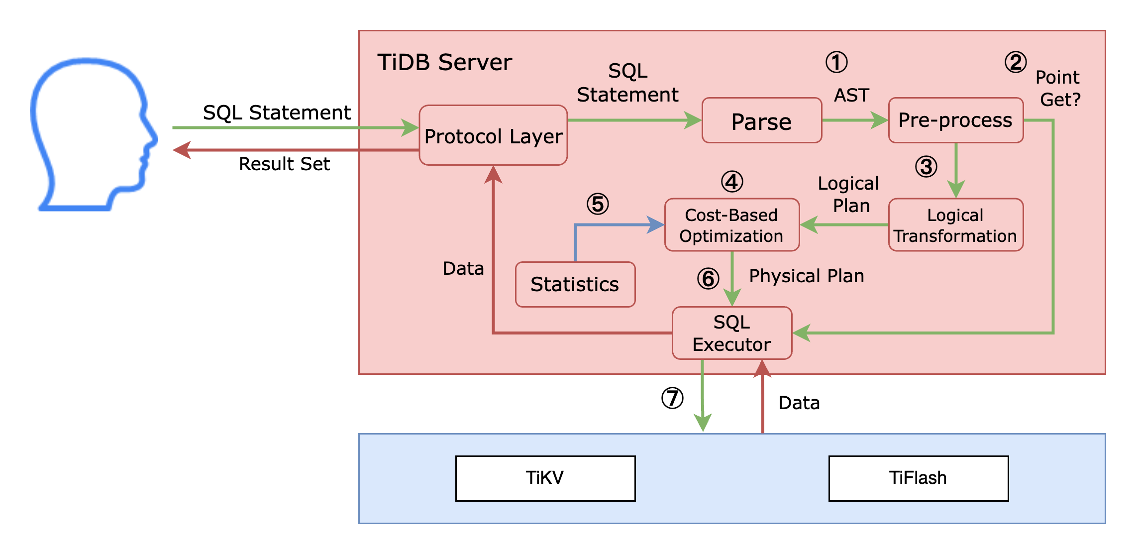
In the preceding figure, to the right of the protocol layer is the optimizer of the TiDB server, which processes SQL statements as follows:
- The SQL statement arrives at the SQL optimizer through the protocol layer and is parsed into an abstract syntax tree (AST).
- TiDB identifies whether it is a Point Get statement, which involves a simple one-table lookup through a primary or unique key, such as
SELECT * FROM t WHERE pk_col = 1orSELECT * FROM t WHERE uk_col IN (1,2,3). ForPoint Getstatements, TiDB skips subsequent optimization steps and proceeds directly to execution in the SQL executor. - If the query is not a
Point Get, the AST undergoes logical transformation, where TiDB rewrites the SQL logically based on specific rules. - After logical transformation, TiDB processes the AST through cost-based optimization.
- During cost-based optimization, the optimizer uses statistics to select appropriate operators and generates a physical execution plan.
- The generated physical execution plan is sent to the SQL executor of the TiDB node for execution.
- Unlike traditional single-node databases, TiDB pushes down operators or coprocessors to TiKV and/or TiFlash nodes containing the data. This approach processes parts of the execution plan where the data is stored, efficiently utilizing the distributed architecture, using resources in parallel, and reducing network data transfer. The TiDB node executor then assembles the final result and returns it to the client.
Optimizer fundamentals
TiDB uses a cost-based optimizer (CBO) to determine the most efficient execution plan for a SQL statement. The optimizer evaluates different execution strategies and selects the one with the lowest estimated cost. The cost depends on factors such as:
- The SQL statement
- Schema design
- Statistics, including:
- Table statistics
- Index statistics
- Column statistics
Based on these inputs, the cost model generates an execution plan that details how TiDB will execute the SQL statement, including:
- Access method
- Join method
- Join order
The effectiveness of the optimizer depends on the quality of the information it receives. To achieve optimal performance, ensure that statistics are up to date and indexes are well-designed.
Statistics management
Statistics are essential for the TiDB optimizer. TiDB uses statistics as the input of the optimizer to estimate the number of rows processed in each step of a SQL execution plan.
Statistics are divided into two levels:
- Table-level statistics: include the total number of rows in the table and the number of rows modified since the last statistics collection.
- Index/column-level statistics: include detailed information such as histograms, Count-Min Sketch, Top-N (values or indexes with the highest occurrences), distribution and quantity of different values, and the number of NULL values.
To check the accuracy and health of your statistics, you can use the following SQL statements:
SHOW STATS_META: shows metadata about table statistics.SHOW STATS_META WHERE table_name='T2'\G;*************************** 1. row *************************** Db_name: test Table_name: T2 Partition_name: Update_time: 2023-05-11 02:16:50 Modify_count: 10000 Row_count: 20000 1 row in set (0.03 sec)SHOW STATS_HEALTHY: shows the health status of table statistics.SHOW STATS_HEALTHY WHERE table_name='T2'\G;*************************** 1. row *************************** Db_name: test Table_name: T2 Partition_name: Healthy: 50 1 row in set (0.00 sec)
TiDB provides two methods for collecting statistics: automatic and manual collection. In most cases, automatic collection is sufficient. TiDB triggers automatic collection when certain conditions are met. Some common triggering conditions include:
tidb_auto_analyze_ratio: the healthiness trigger.tidb_auto_analyze_start_timeandtidb_auto_analyze_end_time: the time window for automatic statistics collection.
SHOW VARIABLES LIKE 'tidb\_auto\_analyze%';
+-----------------------------------------+-------------+
| Variable_name                           | Value       |
+-----------------------------------------+-------------+
| tidb_auto_analyze_ratio                 | 0.5         |
| tidb_auto_analyze_start_time            | 00:00 +0000 |
| tidb_auto_analyze_end_time              | 23:59 +0000 |
+-----------------------------------------+-------------+
In some cases, automatic collection might not meet your needs. By default, it occurs between 00:00 and 23:59, meaning the analyze job can run at any time. To minimize performance impact on your online business, you can set specific start and end times for statistics collection.
You can manually collect statistics using the ANALYZE TABLE table_name statement. This lets you adjust settings such as the sample rate, the number of Top-N values, or collect statistics for specific columns only.
Note that after manual collection, subsequent automatic collection jobs inherit the new settings. This means that any customizations made during manual collection will apply to future automatic analyses.
Locking table statistics is useful in the following scenarios:
- The statistics on the table already represent the data well.
- The table is very large, and statistics collection is time-consuming.
- You want to maintain statistics only during specific time windows.
To lock statistics for a table, you can use the LOCK STATS table_name statement.
For more information, see Statistics.
Understand execution plans
An execution plan details the steps that TiDB will follow to execute a SQL query. This section explains how TiDB builds an execution plan and how to generate, display, and interpret execution plans.
How TiDB builds an execution plan
A SQL statement undergoes three main optimization stages in the TiDB optimizer:
1. Pre-processing
During pre-processing, TiDB determines whether the SQL statement can be executed using Point_Get or Batch_Point_Get. These operations use a primary or unique key to read directly from TiKV through an exact key lookup. If a plan qualifies for Point_Get or Batch_Point_Get, the optimizer skips the logical transformation and cost-based optimization steps because direct key lookup is the most efficient way to access the row.
The following is an example of a Point_Get query:
EXPLAIN SELECT id, name FROM emp WHERE id = 901;
+-------------+---------+------+---------------+---------------+
| id          | estRows | task | access object | operator info |
+-------------+---------+------+---------------+---------------+
| Point_Get_1 | 1.00    | root | table:emp     | handle:901    |
+-------------+---------+------+---------------+---------------+
2. Logical transformation
During logical transformation, TiDB optimizes SQL statements based on the SELECT list, WHERE predicates, and other conditions. It generates a logical execution plan to annotate and rewrite the query. This logical plan is used in the next stage, cost-based optimization. The transformation applies rule-based optimizations such as column pruning, partition pruning, and join reordering. Because this process is rule-based and automatic, manual adjustments are usually unnecessary.
For more information, see SQL Logical Optimization.
3. Cost-based optimization
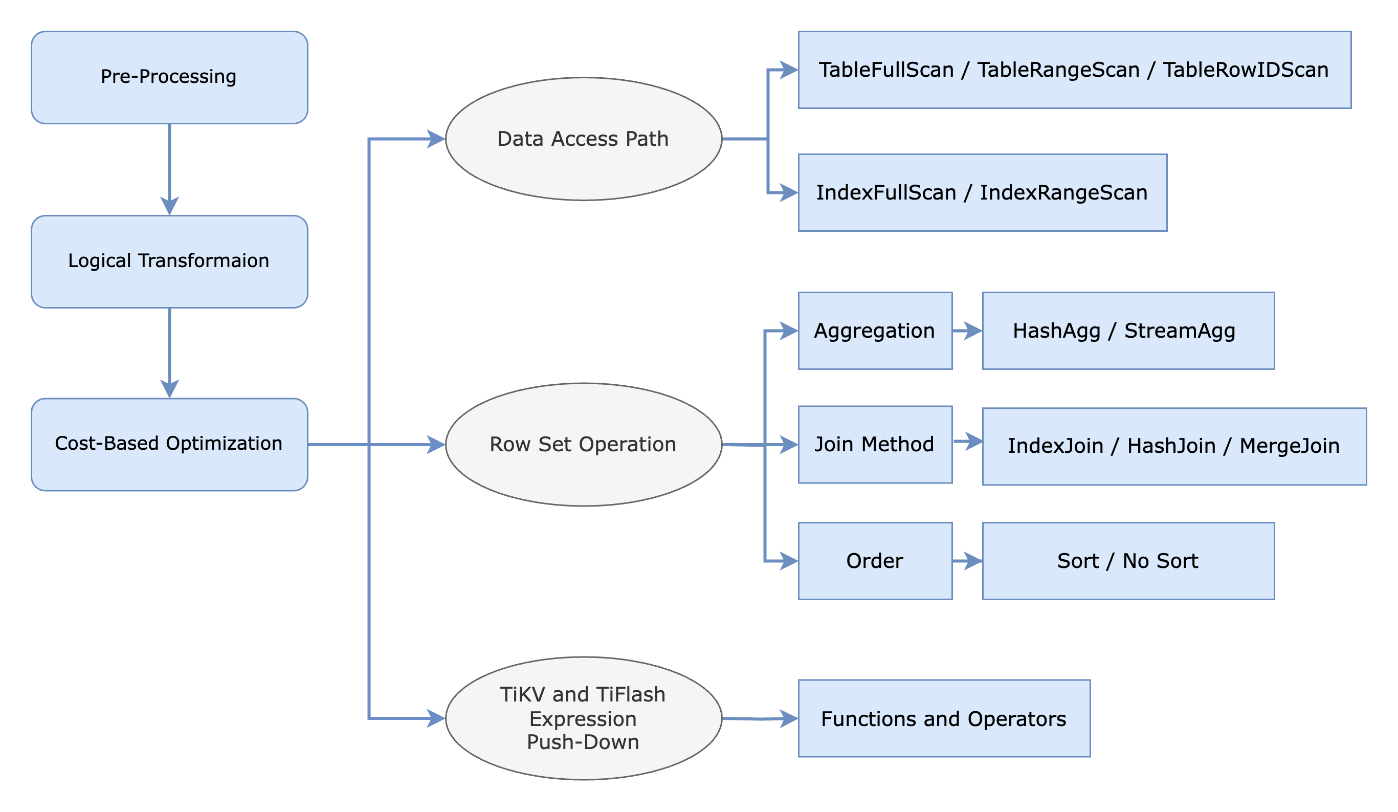
The TiDB optimizer uses statistics to estimate the number of rows processed in each step of a SQL statement and assigns a cost to each step. During cost-based optimization, the optimizer evaluates all possible plan choices, including index accesses and join methods, and calculates the total cost for each plan. The optimizer then selects the execution plan with the minimal total cost.
The following figure illustrates various data access paths and row set operations considered during cost-based optimization. For data retrieval paths, the optimizer determines the most efficient method between index scans and full table scans, and decides whether to retrieve data from row-based TiKV storage or columnar TiFlash storage.
The optimizer also evaluates operations that manipulate row sets, such as aggregation, join, and sorting. For example, the aggregation operator might use either HashAgg or StreamAgg, while the join method can select from HashJoin, MergeJoin, or IndexJoin.
Additionally, the physical optimization phase includes pushing down expressions and operators to the physical storage engines. The physical plan is distributed to different components based on the underlying storage engines as follows:
- Root tasks are executed on the TiDB server.
- Cop (Coprocessor) tasks are executed on TiKV.
- MPP tasks are executed on TiFlash.
This distribution enables cross-component collaboration for efficient query processing.
For more information, see SQL Physical Optimization.
Generate and display execution plans
Besides accessing execution plan information through TiDB Dashboard, you can use the EXPLAIN statement to display the execution plan for a SQL query. The EXPLAIN output includes the following columns:
id: the operator name and a unique identifier of the step.estRows: the estimated number of rows from the particular step.task: indicates the layer where the operator is executed. For example,rootindicates execution on the TiDB server,cop[tikv]indicates execution on TiKV, andmpp[tiflash]indicates execution on TiFlash.access object: the object where row sources are located.operator info: additional details about the operator in the step.
EXPLAIN SELECT COUNT(*) FROM trips WHERE start_date BETWEEN '2017-07-01 00:00:00' AND '2017-07-01 23:59:59';
+--------------------------+-------------+--------------+-------------------+----------------------------------------------------------------------------------------------------+
| id                       | estRows     | task         | access object     | operator info                                                                                      |
+--------------------------+-------------+--------------+-------------------+----------------------------------------------------------------------------------------------------+
| StreamAgg_20             | 1.00        | root         |                   | funcs:count(Column#13)->Column#11                                                                  |
| └─TableReader_21         | 1.00        | root         |                   | data:StreamAgg_9                                                                                   |
|   └─StreamAgg_9          | 1.00        | cop[tikv]    |                   | funcs:count(1)->Column#13                                                                          |
|     └─Selection_19       | 250.00      | cop[tikv]    |                   | ge(trips.start_date, 2017-07-01 00:00:00.000000), le(trips.start_date, 2017-07-01 23:59:59.000000) |
|       └─TableFullScan_18 | 10000.00    | cop[tikv]    | table:trips       | keep order:false, stats:pseudo                                                                     |
+--------------------------+-------------+--------------+-------------------+----------------------------------------------------------------------------------------------------+
5 rows in set (0.00 sec)
Different from EXPLAIN, EXPLAIN ANALYZE executes the corresponding SQL statement, records its runtime information, and returns the runtime information together with the execution plan. This runtime information is crucial for debugging query execution. For more information, see EXPLAIN ANALYZE.
The EXPLAIN ANALYZE output includes:
actRows: the number of rows output by the operator.execution info: detailed execution information of the operator.timerepresents the totalwall time, including the total execution time of all sub-operators. If the operator is called many times by the parent operator, then the time refers to the accumulated time.memory: the memory used by the operator.disk: the disk space used by the operator.
The following is an example. Some attributes and table columns are omitted to improve formatting.
EXPLAIN ANALYZE
SELECT SUM(pm.m_count) / COUNT(*)
FROM (
    SELECT COUNT(m.name) m_count
    FROM universe.moons m
    RIGHT JOIN (
        SELECT p.id, p.name
        FROM universe.planet_categories c
        JOIN universe.planets p
            ON c.id = p.category_id
            AND c.name = 'Jovian'
    ) pc ON m.planet_id = pc.id
    GROUP BY pc.name
) pm;
+-----------------------------------------+.+---------+-----------+---------------------------+----------------------------------------------------------------+.+-----------+---------+
| id                                      |.| actRows | task      | access object             | execution info                                                 |.| memory    | disk    |
+-----------------------------------------+.+---------+-----------+---------------------------+----------------------------------------------------------------+.+-----------+---------+
| Projection_14                           |.| 1       | root      |                           | time:1.39ms, loops:2, RU:1.561975, Concurrency:OFF             |.| 9.64 KB   | N/A     |
| └─StreamAgg_16                          |.| 1       | root      |                           | time:1.39ms, loops:2                                           |.| 1.46 KB   | N/A     |
|   └─Projection_40                       |.| 4       | root      |                           | time:1.38ms, loops:4, Concurrency:OFF                          |.| 8.24 KB   | N/A     |
|     └─HashAgg_17                        |.| 4       | root      |                           | time:1.36ms, loops:4, partial_worker:{...}, final_worker:{...} |.| 82.1 KB   | N/A     |
|       └─HashJoin_19                     |.| 25      | root      |                           | time:1.29ms, loops:2, build_hash_table:{...}, probe:{...}      |.| 2.25 KB   | 0 Bytes |
|         ├─HashJoin_35(Build)            |.| 4       | root      |                           | time:1.08ms, loops:2, build_hash_table:{...}, probe:{...}      |.| 25.7 KB   | 0 Bytes |
|         │ ├─IndexReader_39(Build)       |.| 1       | root      |                           | time:888.5µs, loops:2, cop_task: {...}                         |.| 286 Bytes | N/A     |
|         │ │ └─IndexRangeScan_38         |.| 1       | cop[tikv] | table:c, index:name(name) | tikv_task:{time:0s, loops:1}, scan_detail: {...}               |.| N/A       | N/A     |
|         │ └─TableReader_37(Probe)       |.| 10      | root      |                           | time:543.7µs, loops:2, cop_task: {...}                         |.| 577 Bytes | N/A     |
|         │   └─TableFullScan_36          |.| 10      | cop[tikv] | table:p                   | tikv_task:{time:0s, loops:1}, scan_detail: {...}               |.| N/A       | N/A     |
|         └─TableReader_22(Probe)         |.| 28      | root      |                           | time:671.7µs, loops:2, cop_task: {...}                         |.| 876 Bytes | N/A     |
|           └─TableFullScan_21            |.| 28      | cop[tikv] | table:m                   | tikv_task:{time:0s, loops:1}, scan_detail: {...}               |.| N/A       | N/A     |
+-----------------------------------------+.+---------+-----------+---------------------------+----------------------------------------------------------------+.+-----------+---------+
Read execution plans: first child first
To diagnose slow SQL queries, you need to understand how to read execution plans. The key principle is "first child first – recursive descent". Each operator in the plan generates a set of rows, and the execution order determines how these rows flow through the plan tree.
The "first child first" rule means that an operator must retrieve rows from all its child operators before producing output. For example, a join operator requires rows from both its child operators to perform the join. The "recursive descent" rule means you analyze the plan from top to bottom, although actual data flows from bottom to top, as each operator depends on its children's output.
Consider these two important concepts when reading execution plans:
Parent-child interaction: a parent operator calls its child operators sequentially but might cycle through them multiple times. For example, in an index lookup or nested loop join, the parent fetches a batch of rows from the first child, then retrieves zero or more rows from the second child. This process repeats until the first child's result set is fully processed.
Blocking vs. non-blocking operators: operators can be either blocking or non-blocking:
- Blocking operators, such as
TopNandHashAgg, must create their entire result set before passing data to their parent. - Non-blocking operators, such as
IndexLookupandIndexJoin, produce and pass rows incrementally as needed.
- Blocking operators, such as
When reading an execution plan, start from the top and work downward. In the following example, the leaf node of the plan tree is TableFullScan_18, which performs a full table scan. The rows from this scan are consumed by the Selection_19 operator, which filters the data based on ge(trips.start_date, 2017-07-01 00:00:00.000000), le(trips.start_date, 2017-07-01 23:59:59.000000). Then, the group-by operator StreamAgg_9 performs the final aggregation COUNT(*).
These three operators (TableFullScan_18, Selection_19, and StreamAgg_9) are pushed down to TiKV (marked as cop[tikv]), enabling early filtering and aggregation in TiKV to reduce data transfer between TiKV and TiDB. Finally, TableReader_21 reads the data from StreamAgg_9, and StreamAgg_20 performs the final aggregation count(*).
EXPLAIN SELECT COUNT(*) FROM trips WHERE start_date BETWEEN '2017-07-01 00:00:00' AND '2017-07-01 23:59:59';
+--------------------------+-------------+--------------+-------------------+----------------------------------------------------------------------------------------------------+
| id                       | estRows     | task         | access object     | operator info                                                                                      |
+--------------------------+-------------+--------------+-------------------+----------------------------------------------------------------------------------------------------+
| StreamAgg_20             | 1.00        | root         |                   | funcs:count(Column#13)->Column#11                                                                  |
| └─TableReader_21         | 1.00        | root         |                   | data:StreamAgg_9                                                                                   |
|   └─StreamAgg_9          | 1.00        | cop[tikv]    |                   | funcs:count(1)->Column#13                                                                          |
|     └─Selection_19       | 250.00      | cop[tikv]    |                   | ge(trips.start_date, 2017-07-01 00:00:00.000000), le(trips.start_date, 2017-07-01 23:59:59.000000) |
|       └─TableFullScan_18 | 10000.00    | cop[tikv]    | table:trips       | keep order:false, stats:pseudo                                                                     |
+--------------------------+-------------+--------------+-------------------+----------------------------------------------------------------------------------------------------+
5 rows in set (0.00 sec)
In the following example, start by examining IndexRangeScan_47, the first leaf node of the plan tree. The optimizer selects only the name and id columns from the stars table, which can be retrieved from the name(name) index. As a result, the root reader for stars is IndexReader_48, not TableReader.
The join between stars and planets is a hash join (HashJoin_44). The planets table is accessed using a full table scan (TableFullScan_45). After the join, TopN_26 and TopN_19 apply the ORDER BY and LIMIT clauses, respectively. The final operator, Projection_16, selects the final column t5.name.
EXPLAIN
SELECT t5.name
FROM (
    SELECT p.name, p.gravity, p.distance_from_sun
    FROM universe.planets p
    JOIN universe.stars s
        ON s.id = p.sun_id
        AND s.name = 'Sun'
    ORDER BY p.distance_from_sun ASC
    LIMIT 5
) t5
ORDER BY t5.gravity DESC
LIMIT 3;
+-----------------------------------+----------+-----------+---------------------------+
| id                                | estRows  | task      | access object             |
+-----------------------------------+----------+-----------+---------------------------+
| Projection_16                     | 3.00     | root      |                           |
| └─TopN_19                         | 3.00     | root      |                           |
|   └─TopN_26                       | 5.00     | root      |                           |
|     └─HashJoin_44                 | 5.00     | root      |                           |
|       ├─IndexReader_48(Build)     | 1.00     | root      |                           |
|       │ └─IndexRangeScan_47       | 1.00     | cop[tikv] | table:s, index:name(name) |
|       └─TableReader_46(Probe)     | 10.00    | root      |                           |
|         └─TableFullScan_45        | 10.00    | cop[tikv] | table:p                   |
+-----------------------------------+----------+-----------+---------------------------+
The following figure illustrates the plan tree for the second execution plan:
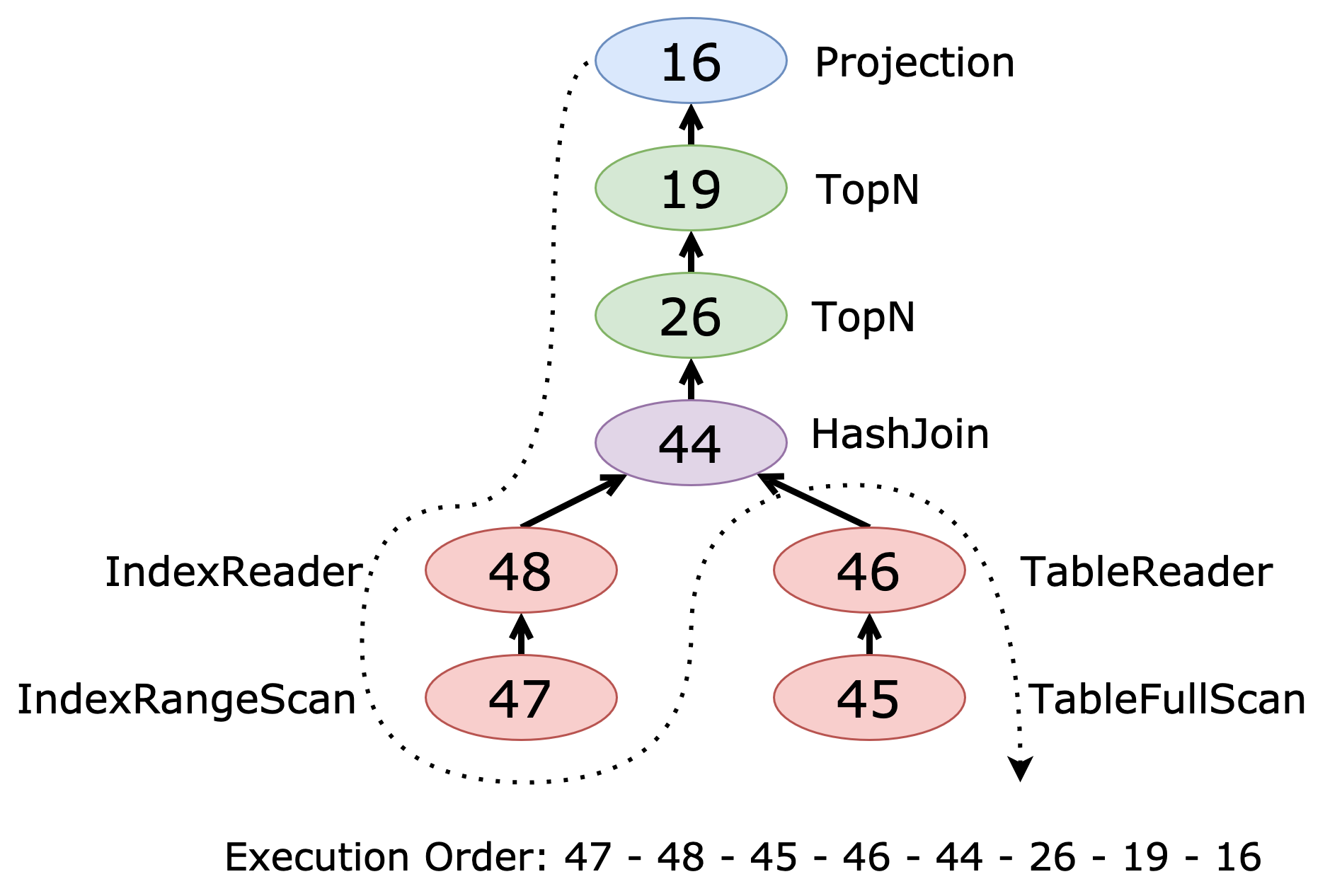
The execution plan follows a top-to-bottom, first-child-first traversal, corresponding to a postorder traversal (Left, Right, Root) of the plan tree.
You can read this plan in the following order:
- Start at the top with
Projection_16. - Move to its child,
TopN_19. - Continue to
TopN_26. - Proceed to
HashJoin_44. - For
HashJoin_44, process its left (Build) child first:IndexReader_48IndexRangeScan_47
- For
HashJoin_44, process its right (Probe) child:TableReader_46TableFullScan_45
This traversal ensures that each operator's inputs are processed before the operator itself, enabling efficient query execution.
Identify bottlenecks in execution plans
When analyzing execution plans, compare actRows (actual rows) with estRows (estimated rows) to evaluate the accuracy of the optimizer's estimations. A significant difference between these values might indicate outdated or inaccurate statistics, which can lead to suboptimal query plans.
To identify bottlenecks in a slow query, perform the following steps:
- Review the
execution infosection from top to bottom, focusing on operators with high execution time. - For the first child operator that consumes significant time:
- Compare
actRowswithestRowsto assess estimation accuracy. - Analyze detailed metrics in
execution info, such as high execution time or other metrics. - Check
memoryanddiskusage for potential resource constraints.
- Compare
- Correlate these factors to determine the root cause of the performance issue. For example, if a
TableFullScanoperation has a highactRowscount and long execution time inexecution info, consider creating an index. If aHashJoinoperation shows high memory usage and execution time, consider optimizing the join order or using an alternative join method.
In the following execution plan, the query runs for 5 minutes and 51 seconds before being canceled. The key issues include:
- Severe underestimation: The first leaf node
IndexReader_76reads data from theindex_orders_on_adjustment_id(adjustment_id)index. The actual number of rows (actRows) is 256,811,189, which is significantly higher than the estimated 1 row (estRows). - Memory overflow: This underestimation causes the hash join operator
HashJoin_69to build a hash table with far more data than expected, consuming excessive memory (22.6 GB) and disk space (7.65 GB). - Query termination: The
actRowsvalue of0forHashJoin_69and operators above it indicate either no matching rows or query termination due to resource constraints. In this case, the hash join consumes too much memory, triggering memory control mechanisms to terminate the query. - Incorrect join order: The root cause of this inefficient plan is the severe underestimation of
estRowsforIndexRangeScan_75, leading the optimizer to choose an incorrect join order.
To address these issues, ensure that table statistics are up to date, particularly for the orders table and the index_orders_on_adjustment_id index.
+-------------------------------------------------------------------------------------------------------------------------------------------------------------------------------------------------...----------------------+
| id                                 | estRows   | estCost      | actRows   | task      | access object                                                                          | execution info ...| memory   | disk     |
+-------------------------------------------------------------------------------------------------------------------------------------------------------------------------------------------------...----------------------+
| TopN_19                            | 1.01      | 461374372.63 | 0         | root      |                                                                                        | time:5m51.1s, l...| 0 Bytes  | 0 Bytes  |
| └─IndexJoin_32                     | 1.01      | 460915067.45 | 0         | root      |                                                                                        | time:5m51.1s, l...| 0 Bytes  | N/A      |
|   ├─HashJoin_69(Build)             | 1.01      | 460913065.41 | 0         | root      |                                                                                        | time:5m51.1s, l...| 21.6 GB  | 7.65 GB  |
|   │ ├─IndexReader_76(Build)        | 1.00      | 18.80        | 256805045 | root      |                                                                                        | time:1m4.1s, lo...| 12.4 MB  | N/A      |
|   │ │ └─IndexRangeScan_75          | 1.00      | 186.74       | 256811189 | cop[tikv] | table:orders, index:index_orders_on_adjustment_id(adjustment_id)                       | tikv_task:{proc...| N/A      | N/A      |
|   │ └─Projection_74(Probe)         | 30652.93  | 460299612.60 | 1024      | root      |                                                                                        | time:1.08s, loo...| 413.4 KB | N/A      |
|   │   └─IndexLookUp_73             | 30652.93  | 460287375.95 | 6144      | root      | partition:all                                                                          | time:1.08s, loo...| 107.8 MB | N/A      |
|   │     ├─IndexRangeScan_70(Build) | 234759.64 | 53362737.50  | 390699    | cop[tikv] | table:rates, index:index_rates_on_label_id(label_id)                                   | time:29.6ms, lo...| N/A      | N/A      |
|   │     └─Selection_72(Probe)      | 30652.93  | 110373973.91 | 187070    | cop[tikv] |                                                                                        | time:36.8s, loo...| N/A      | N/A      |
|   │       └─TableRowIDScan_71      | 234759.64 | 86944962.10  | 390699    | cop[tikv] | table:rates                                                                            | tikv_task:{proc...| N/A      | N/A      |
|   └─TableReader_28(Probe)          | 0.00      | 43.64        | 0         | root      |                                                                                        |                ...| N/A      | N/A      |
|     └─Selection_27                 | 0.00      | 653.96       | 0         | cop[tikv] |                                                                                        |                ...| N/A      | N/A      |
|       └─TableRangeScan_26          | 1.01      | 454.36       | 0         | cop[tikv] | table:labels                                                                           |                ...| N/A      | N/A      |
+-------------------------------------------------------------------------------------------------------------------------------------------------------------------------------------------------...----------------------+
The following execution plan shows the expected results after fixing the incorrect estimation on the orders table. The query now takes 1.96 seconds to run, which is a significant improvement from the previous 5 minutes and 51 seconds:
- Accurate estimation: The
estRowsvalues now closely match theactRows, indicating that the statistics are updated and more accurate. - Efficient join order: The query now starts with a
TableReaderon thelabelstable, followed by anIndexJoinwith theratestable, and anotherIndexJoinwith theorderstable. This join order works more efficiently with the actual data distribution. - No memory overflow: Unlike the previous plan, this execution shows no signs of excessive memory or disk usage, indicating that the query runs within expected resource limits.
This optimized plan demonstrates the importance of accurate statistics and proper join order in query performance. The execution time reduction (from 351 seconds to 1.96 seconds) shows the impact of addressing estimation errors.
+---------------------------------------+----------+---------+-----------+----------------------------------------------------------------------------------------+---------------...+----------+------+
| id                                    | estRows  | actRows | task      | access object                                                                          | execution info...| memory   | disk |
+---------------------------------------+----------+---------+-----------+----------------------------------------------------------------------------------------+---------------...+----------+------+
| Limit_24                              | 1000.00  | 1000    | root      |                                                                                        | time:1.96s, lo...| N/A      | N/A  |
| └─IndexJoin_88                        | 1000.00  | 1000    | root      |                                                                                        | time:1.96s, lo...| 1.32 MB  | N/A  |
|   ├─IndexJoin_99(Build)               | 1000.00  | 2458    | root      |                                                                                        | time:1.96s, lo...| 77.7 MB  | N/A  |
|   │ ├─TableReader_109(Build)          | 6505.62  | 158728  | root      |                                                                                        | time:1.26s, lo...| 297.0 MB | N/A  |
|   │ │ └─Selection_108                 | 6505.62  | 171583  | cop[tikv] |                                                                                        | tikv_task:{pro...| N/A      | N/A  |
|   │ │   └─TableRangeScan_107          | 80396.43 | 179616  | cop[tikv] | table:labels                                                                           | tikv_task:{pro...| N/A      | N/A  |
|   │ └─Projection_98(Probe)            | 1000.00  | 2458    | root      |                                                                                        | time:2.13s, lo...| 59.2 KB  | N/A  |
|   │   └─IndexLookUp_97                | 1000.00  | 2458    | root      | partition:all                                                                          | time:2.13s, lo...| 1.20 MB  | N/A  |
|   │     ├─Selection_95(Build)         | 6517.14  | 6481    | cop[tikv] |                                                                                        | time:798.6ms, ...| N/A      | N/A  |
|   │     │ └─IndexRangeScan_93         | 6517.14  | 6481    | cop[tikv] | table:rates, index:index_rates_on_label_id(label_id)                                   | tikv_task:{pro...| N/A      | N/A  |
|   │     └─Selection_96(Probe)         | 1000.00  | 2458    | cop[tikv] |                                                                                        | time:444.4ms, ...| N/A      | N/A  |
|   │       └─TableRowIDScan_94         | 6517.14  | 6481    | cop[tikv] | table:rates                                                                            | tikv_task:{pro...| N/A      | N/A  |
|   └─TableReader_84(Probe)             | 984.56   | 1998    | root      |                                                                                        | time:207.6ms, ...| N/A      | N/A  |
|     └─Selection_83                    | 984.56   | 1998    | cop[tikv] |                                                                                        | tikv_task:{pro...| N/A      | N/A  |
|       └─TableRangeScan_82             | 1000.00  | 2048    | cop[tikv] | table:orders                                                                           | tikv_task:{pro...| N/A      | N/A  |
+---------------------------------------+----------+---------+-----------+----------------------------------------------------------------------------------------+---------------...+----------+------+
For more information, see TiDB Query Execution Plan Overview and EXPLAIN Walkthrough.
Index strategy in TiDB
TiDB is a distributed SQL database that separates the SQL layer (TiDB Server) from the storage layer (TiKV). Unlike traditional databases, TiDB does not use a buffer pool to cache data on compute nodes. As a result, SQL query performance and overall cluster performance depend on the number of key-value (KV) RPC requests that need to be processed. Common KV RPC requests include Point_Get, Batch_Point_Get, and Coprocessor.
To optimize performance in TiDB, it is essential to use indexes effectively, as they can significantly reduce the number of KV RPC requests. Fewer KV RPC requests improve query performance and system efficiency. The following lists some key strategies that help optimize indexing:
- Avoid full table scans.
- Avoid sorting operations.
- Use covering indexes or exclude unnecessary columns to reduce row lookups.
This section explains general indexing strategies and indexing costs. It also provides three practical examples of effective indexing in TiDB, with a focus on composite and covering indexes for SQL tuning.
Composite index strategy guidelines
To create an efficient composite index, order your columns strategically. The column order directly affects how efficiently the index filters and sorts data.
Follow these recommended column order guidelines for a composite index:
Start with index prefix columns for direct access:
- Columns with equivalent conditions
- Columns with
IS NULLconditions - Columns with
INconditions that contain a single value, such asIN (1)
Add columns for sorting next:
- Let the index handle sorting operations
- Enable sort and limit pushdown to TiKV
- Preserve the sorted order
Include additional filtering columns to reduce row lookups:
INconditions with multiple values- Time range conditions on datetime columns
- Other non-equivalent conditions, such as
!=,<>,NOT IN, andIS NOT NULL
Add columns from the
SELECTlist or used in aggregation to fully utilize a covering index.
Special consideration: IN conditions
When designing composite indexes, you need to handle IN conditions carefully.
- Single value: an
INclause with a single value (such asIN (1)) works similarly to an equality condition and can be placed at the beginning of the index. - Multiple values: an
INclause with multiple values generates multiple ranges. If you place such a column before columns used for sorting, it can break the sorting order. To maintain the sorting order, make sure to place columns used for sorting before columns with multi-valueINconditions in the composite index.
The cost of indexing
While indexes can improve query performance, they also introduce costs you should consider:
Performance impact on writes:
- A non-clustered index reduces the chance of single-phase commit optimization.
- Each additional index slows down write operations (such as
INSERT,UPDATE, andDELETE). - When data is modified, all affected indexes must be updated.
- The more indexes a table has, the greater the write performance impact.
Resource consumption:
- Indexes require additional disk space.
- More memory is needed to cache frequently accessed indexes.
- Backup and recovery operations take longer.
Write hotspot risk:
- Secondary indexes can create write hotspots. For example, a monotonically increasing datetime index will cause hotspots on table writes.
- Hotspots can lead to significant performance degradation.
The following lists some best practices:
- Create indexes only when they provide clear performance benefits.
- Regularly review index usage statistics using
TIDB_INDEX_USAGE. - Consider the write/read ratio of your workload when designing indexes.
SQL tuning with a covering index
A covering index includes all columns referenced in the WHERE and SELECT clauses. Using a covering index can eliminate the need for additional index lookups, significantly improving query performance.
The following query requires an index lookup of 2,597,411 rows and takes 46.4 seconds to execute. TiDB dispatches 67 cop tasks for the index range scan on logs_idx (IndexRangeScan_11) and 301 cop tasks for table access (TableRowIDScan_12).
SELECT
  SUM(`logs`.`amount`)
FROM
  `logs`
WHERE
  `logs`.`user_id` = 1111
  AND `logs`.`snapshot_id` IS NULL
  AND `logs`.`status` IN ('complete', 'failure')
  AND `logs`.`source_type` != 'online'
  AND (
    `logs`.`source_type` IN ('user', 'payment')
    OR `logs`.`source_type` IN (
      'bank_account',
    )
    AND `logs`.`target_type` IN ('bank_account')
  );
The original execution plan is as follows:
+-------------------------------+------------+---------+-----------+--------------------------------------------------------------------------+------------------------------------------------------------+
| id                            | estRows    | actRows | task      | access object                                                            | execution info                                             |
+-------------------------------+------------+---------+-----------+--------------------------------------------------------------------------+------------------------------------------------------------+
| HashAgg_18                   | 1.00       | 2571625.22 | 1       | root      |                                                              | time:46.4s, loops:2, partial_worker:{wall_time:46.37,   ...|
| └─IndexLookUp_19             | 1.00       | 2570096.68 | 301     | root      |                                                              | time:46.4s, loops:2, index_task: {total_time: 45.8s,    ...|
|   ├─IndexRangeScan_11(Build) | 1309.50    | 317033.98  | 2597411 | cop[tikv] | table:logs, index:logs_idx(snapshot_id, user_id, status)     | time:228ms, loops:2547, cop_task: {num: 67, max: 2.17s, ...|
|   └─HashAgg_7(Probe)         | 1.00       | 588434.48  | 301     | cop[tikv] |                                                              | time:3m46.7s, loops:260, cop_task: {num: 301,           ...|
|     └─Selection_13           | 1271.37    | 561549.27  | 2566562 | cop[tikv] |                                                              | tikv_task:{proc max:10s, min:0s, avg: 915.3ms,          ...|
|       └─TableRowIDScan_12    | 1309.50    | 430861.31  | 2597411 | cop[tikv] | table:logs                                                   | tikv_task:{proc max:10s, min:0s, avg: 908.7ms,          ...|
+-------------------------------+------------+---------+-----------+--------------------------------------------------------------------------+------------------------------------------------------------+
To improve query performance, you can create a covering index that includes source_type, target_type, and amount columns. This optimization eliminates the need for additional table lookups, reducing execution time to 90 milliseconds, and TiDB only needs to send one cop task to TiKV for data scanning.
After creating the index, execute the ANALYZE TABLE statement to collect statistics. In TiDB, index creation does not automatically update statistics, so analyzing the table ensures that the optimizer selects the new index.
CREATE INDEX logs_covered ON logs(snapshot_id, user_id, status, source_type, target_type, amount);
ANALYZE TABLE logs INDEX logs_covered;
The new execution plan is as follows:
+-------------------------------+------------+---------+-----------+---------------------------------------------------------------------------------------------------------------------------------+---------------------------------------------+
| id                            | estRows    | actRows | task      | access object                                                                                                                   | execution info                              |
+-------------------------------+------------+---------+-----------+---------------------------------------------------------------------------------------------------------------------------------+---------------------------------------------+
| HashAgg_13                    | 1.00       | 1       | root      |                                                                                                                                 | time:90ms, loops:2, RU:158.885311,       ...|
| └─IndexReader_14              | 1.00       | 1       | root      |                                                                                                                                 | time:89.8ms, loops:2, cop_task: {num: 1, ...|
|   └─HashAgg_6                 | 1.00       | 1       | cop[tikv] |                                                                                                                                 | tikv_task:{time:88ms, loops:52},         ...|
|     └─Selection_12            | 5245632.33 | 52863   | cop[tikv] |                                                                                                                                 | tikv_task:{time:80ms, loops:52}          ...|
|       └─IndexRangeScan_11     | 5245632.33 | 52863   | cop[tikv] | table:logs, index:logs_covered(snapshot_id, user_id, status, source_type, target_type, amount)                                  | tikv_task:{time:60ms, loops:52}          ...|
+-------------------------------+------------+---------+-----------+---------------------------------------------------------------------------------------------------------------------------------+---------------------------------------------+
SQL tuning with a composite index involving sorting
You can optimize queries with ORDER BY clauses by creating composite indexes that include both filtering and sorting columns. This approach helps TiDB access data efficiently while maintaining the desired order.
For example, consider the following query that retrieves data from test based on specific conditions:
EXPLAIN ANALYZE SELECT
test.*
FROM
  test
WHERE
  test.snapshot_id = 459840
  AND test.id > 998464
ORDER BY
  test.id ASC
LIMIT
  1000
The execution plan shows a duration of 170 ms. TiDB uses the test_index to perform an IndexRangeScan_20 with the filter snapshot_id = 459840. It then retrieves all columns from the table, returning 5,715 rows to TiDB after IndexLookUp_23. TiDB sorts these rows and returns 1,000 rows.
The id column is the primary key, which means it is implicitly included in the test_idx index. However, IndexRangeScan_20 does not guarantee order because test_idx includes two additional columns (user_id and status) after the index prefix column snapshot_id. As a result, the ordering of id is not preserved.
The original plan is as follows:
+------------------------------+---------+---------+-----------+----------------------------------------------------------+-----------------------------------------------+--------------------------------------------+
| id                           | estRows | actRows | task      | access object                                            | execution info                                | operator info                              |
+------------------------------+---------+---------+-----------+----------------------------------------------------------+-----------------------------------------------+--------------------------------------------+
| id                           | estRows | actRows | task      | access object                                            | execution info                             ...| test.id, offset:0, count:1000              |
| TopN_10                      | 19.98   | 1000    | root      |                                                          | time:170.6ms, loops:2                      ...|                                            |
| └─IndexLookUp_23             | 19.98   | 5715    | root      |                                                          | time:166.6ms, loops:7                      ...|                                            |
|   ├─Selection_22(Build)      | 19.98   | 5715    | cop[tikv] |                                                          | time:18.6ms, loops:9, cop_task: {num: 3,   ...| gt(test.id, 998464)                        |
|   │ └─IndexRangeScan_20      | 433.47  | 7715    | cop[tikv] | table:test, index:test_idx(snapshot_id, user_id, status) | tikv_task:{proc max:4ms, min:4ms, avg: 4ms ...| range:[459840,459840], keep order:false    |
|   └─TableRowIDScan_21(Probe) | 19.98   | 5715    | cop[tikv] | table:test                                               | time:301.6ms, loops:10, cop_task: {num: 3, ...| keep order:false                           |
+------------------------------+---------+---------+-----------+----------------------------------------------------------+-----------------------------------------------+--------------------------------------------+
To optimize the query, you can create a new index on (snapshot_id). This ensures that id is sorted within each snapshot_id group. With this index, execution time drops to 96 ms. The keep order property becomes true for IndexRangeScan_33, and TopN is replaced with Limit. As a result, IndexLookUp_35 returns only 1,000 rows to TiDB, eliminating the need for additional sorting operations.
The following is the query statement with the optimized index:
CREATE INDEX test_new ON test(snapshot_id);
ANALYZE TABLE test INDEX test_new;
The new plan is as follows:
+----------------------------------+---------+---------+-----------+----------------------------------------------+----------------------------------------------+----------------------------------------------------+
| id                               | estRows | actRows | task      | access object                                | execution info                               | operator info                                      |
+----------------------------------+---------+---------+-----------+----------------------------------------------+----------------------------------------------+----------------------------------------------------+
| Limit_14                         | 17.59   | 1000    | root      |                                              | time:96.1ms, loops:2, RU:92.300155           | offset:0, count:1000                               |
| └─IndexLookUp_35                 | 17.59   | 1000    | root      |                                              | time:96.1ms, loops:1, index_task:         ...|                                                    |
|   ├─IndexRangeScan_33(Build)     | 17.59   | 5715    | cop[tikv] | table:test, index:test_new(snapshot_id)      | time:7.25ms, loops:8, cop_task: {num: 3,  ...| range:(459840 998464,459840 +inf], keep order:true |
|   └─TableRowIDScan_34(Probe)     | 17.59   | 5715    | cop[tikv] | table:test                                   | time:232.9ms, loops:9, cop_task: {num: 3, ...| keep order:false                                   |
+----------------------------------+---------+---------+-----------+----------------------------------------------+----------------------------------------------+----------------------------------------------------+
SQL tuning with composite indexes for efficient filtering and sorting
The following query takes 11 minutes and 9 seconds to execute, which is excessively long for a query that returns only 101 rows. The slow performance is caused by several factors:
- Inefficient index usage: The optimizer selects the index on
created_at, resulting in a scan of 25,147,450 rows. - Large intermediate result set: After applying the date range filter, 12,082,311 rows still require processing.
- Late filtering: The most selective predicates
(mode, user_id, and label_id)are applied after accessing the table, resulting in 16,604 rows. - Sorting overhead: The final sort operation on 16,604 rows adds additional processing time.
The following is the query statement:
SELECT `orders`.*
FROM `orders`
WHERE
    `orders`.`mode` = 'production'
    AND `orders`.`user_id` = 11111
    AND orders.label_id IS NOT NULL
    AND orders.created_at >= '2024-04-07 18:07:52'
    AND orders.created_at <= '2024-05-11 18:07:52'
    AND orders.id >= 1000000000
    AND orders.id < 1500000000
ORDER BY orders.id DESC
LIMIT 101;
The following are the existing indexes on orders:
PRIMARY KEY (`id`),
UNIQUE KEY `index_orders_on_adjustment_id` (`adjustment_id`),
KEY `index_orders_on_user_id` (`user_id`),
KEY `index_orders_on_label_id` (`label_id`),
KEY `index_orders_on_created_at` (`created_at`)
The original execution plan is as follows:
+--------------------------------+-----------+---------+-----------+--------------------------------------------------------------------------------+-----------------------------------------------------+----------------------------------------------------------------------------------------+----------+------+
| id                             | estRows   | actRows | task      | access object                                                                  | execution info                                      | operator info                                                                          | memory   | disk |
+--------------------------------+-----------+---------+-----------+--------------------------------------------------------------------------------+-----------------------------------------------------+----------------------------------------------------------------------------------------+----------+------+
| TopN_10                        | 101.00    | 101     | root      |                                                                                | time:11m9.8s, loops:2                               | orders.id:desc, offset:0, count:101                                                    | 271 KB   | N/A  |
| └─IndexLookUp_39               | 173.83    | 16604   | root      |                                                                                | time:11m9.8s, loops:19, index_task: {total_time:...}|                                                                                        | 20.4 MB  | N/A  |
|   ├─Selection_37(Build)        | 8296.70   | 12082311| cop[tikv] |                                                                                | time:26.4ms, loops:11834, cop_task: {num: 294, m...}| ge(orders.id, 1000000000), lt(orders.id, 1500000000)                                   | N/A      | N/A  |
|   │ └─IndexRangeScan_35        | 6934161.90| 25147450| cop[tikv] | table:orders, index:index_orders_on_created_at(created_at)                     | tikv_task:{proc max:2.15s, min:0s, avg: 58.9ms, ...}| range:[2024-04-07 18:07:52,2024-05-11 18:07:52), keep order:false                      | N/A      | N/A  |
|   └─Selection_38(Probe)        | 173.83    | 16604   | cop[tikv] |                                                                                | time:54m46.2s, loops:651, cop_task: {num: 1076, ...}| eq(orders.mode, "production"), eq(orders.user_id, 11111), not(isnull(orders.label_id)) | N/A      | N/A  |
|     └─TableRowIDScan_36        | 8296.70   | 12082311| cop[tikv] | table:orders                                                                   | tikv_task:{proc max:44.8s, min:0s, avg: 3.33s, p...}| keep order:false                                                                       | N/A      | N/A  |
+--------------------------------+-----------+---------+-----------+--------------------------------------------------------------------------------+-----------------------------------------------------+----------------------------------------------------------------------------------------+----------+------+
After creating a composite index idx_composite on orders(user_id, mode, id, created_at, label_id), the query performance improves significantly. The execution time drops from 11 minutes and 9 seconds to just 5.3 milliseconds, making the query over 126,000 times faster. This massive improvement results from:
- Efficient index usage: the new index enables an index range scan on
user_id,mode, andid, which are the most selective predicates. This reduces the number of scanned rows from millions to just 224. - Index-only sort: the
keep order:truein the execution plan indicates that sorting is performed using the index structure, eliminating the need for a separate sort operation. - Early filtering: the most selective predicates are applied first, reducing the result set to 224 rows before further filtering.
- Limit push-down: the
LIMITclause is pushed down to the index scan, allowing early termination of the scan once 101 rows are found.
This case demonstrates the significant impact of a well-designed index on query performance. By aligning the index structure with the query's predicates, sort order, and required columns, the query achieves a performance improvement of over five orders of magnitude.
CREATE INDEX idx_composite ON orders(user_id, mode, id, created_at, label_id);
ANALYZE TABLE orders index idx_composite;
The new execution plan is as follows:
+--------------------------------+-----------+---------+-----------+--------------------------------------------------------------------------------+-----------------------------------------------------+----------------------------------------------------------------------------------------------------------------------+----------+------+
| id                             | estRows   | actRows | task      | access object                                                                  | execution info                                      | operator info                                                                                                        | memory   | disk |
+--------------------------------+-----------+---------+-----------+--------------------------------------------------------------------------------+-----------------------------------------------------+----------------------------------------------------------------------------------------------------------------------+----------+------+
| IndexLookUp_32                 | 101.00    | 101     | root      |                                                                                | time:5.3ms, loops:2, RU:3.435006, index_task: {t...}| limit embedded(offset:0, count:101)                                                                                  | 128.5 KB | N/A  |
| ├─Limit_31(Build)              | 101.00    | 101     | cop[tikv] |                                                                                | time:1.35ms, loops:1, cop_task: {num: 1, max: 1....}| offset:0, count:101                                                                                                  | N/A      | N/A  |
| │ └─Selection_30               | 535.77    | 224     | cop[tikv] |                                                                                | tikv_task:{time:0s, loops:3}                        | ge(orders.created_at, 2024-04-07 18:07:52), le(orders.created_at, 2024-05-11 18:07:52), not(isnull(orders.label_id)) | N/A      | N/A  |
| │   └─IndexRangeScan_28        | 503893.42 | 224     | cop[tikv] | table:orders, index:idx_composite(user_id, mode, id, created_at, label_id)     | tikv_task:{time:0s, loops:3}                        | range:[11111 "production" 1000000000,11111 "production" 1500000000), keep order:true, desc                           | N/A      | N/A  |
| └─TableRowIDScan_29(Probe)     | 101.00    | 101     | cop[tikv] | table:orders                                                                   | time:2.9ms, loops:2, cop_task: {num: 3, max: 2.7...}| keep order:false                                                                                                     | N/A      | N/A  |
+--------------------------------+-----------+---------+-----------+--------------------------------------------------------------------------------+-----------------------------------------------------+----------------------------------------------------------------------------------------------------------------------+----------+------+
When to use TiFlash
This section explains when to use TiFlash in TiDB. TiFlash is optimized for analytical queries that involve complex calculations, aggregations, and large dataset scans. Its columnar storage format and MPP mode significantly improve performance in these scenarios.
Use TiFlash in the following scenarios:
- Large-scale data analysis: TiFlash delivers faster performance for OLAP workloads that require extensive data scans. Its columnar storage and MPP execution mode optimize query efficiency compared to TiKV.
- Complex scans, aggregations, and joins: TiFlash processes queries with heavy aggregations and joins more efficiently by reading only the necessary columns.
- Mixed workloads: in hybrid environments where both transactional (OLTP) and analytical (OLAP) workloads run simultaneously, TiFlash handles analytical queries without affecting TiKV's performance for transactional queries.
- SaaS applications with arbitrary filtering requirements: queries often involve filtering across many columns. Indexing all columns is impractical, especially when queries include a tenant ID as part of the primary key. TiFlash sorts and clusters data by primary key, making it well suited for these workloads. With the late materialization feature, TiFlash enables efficient table range scans, improving query performance without the overhead of maintaining multiple indexes.
Using TiFlash strategically enhances query performance and optimizes resource usage in TiDB for data-intensive analytical queries. The following sections provide examples of TiFlash use cases.
Analytical query
This section compares the execution performance of TPC-H Query 14 on TiKV and TiFlash storage engines.
TPC-H Query 14 involves joining the order_line and item tables. The query takes 21.1 seconds on TiKV but only 1.41 seconds using TiFlash MPP mode, making it 15 times faster.
- TiKV plan: TiDB fetches 3,864,397 rows from the
lineitemtable and 10 million rows from theparttable. The hash join operation (HashJoin_21), along with the subsequent projection (Projection_38) and aggregation (HashAgg_9) operations, are performed in TiDB. - TiFlash plan: The optimizer detects TiFlash replicas for both
order_lineanditemtables. Based on cost estimation, TiDB automatically selects the MPP mode, executing the entire query within the TiFlash columnar storage engine. This includes table scans, hash joins, column projections, and aggregations, significantly improving performance compared to the TiKV plan.
The following is the query:
select 100.00 * sum(case when i_data like 'PR%' then ol_amount else 0 end) / (1+sum(ol_amount)) as promo_revenue
from order_line, item
where ol_i_id = i_id and ol_delivery_d >= '2007-01-02 00:00:00.000000' and ol_delivery_d < '2030-01-02 00:00:00.000000';
The execution plan on TiKV is as follows:
+-------------------------------+--------------+-----------+-----------+----------------+----------------------------------------------+
| ID                            | ESTROWS      | ACTROWS   | TASK      | ACCESS OBJECT  | EXECUTION INFO                               |
+-------------------------------+--------------+-----------+-----------+----------------+----------------------------------------------+
| Projection_8                  | 1.00         | 1         | root      |                | time:21.1s, loops:2, RU:1023225.707561, ...  |
| └─HashAgg_9                   | 1.00         | 1         | root      |                | time:21.1s, loops:2, partial_worker:{ ...    |
|   └─Projection_38             | 3839984.46   | 3864397   | root      |                | time:21.1s, loops:3776, Concurrency:5        |
|     └─HashJoin_21             | 3839984.46   | 3864397   | root      |                | time:21.1s, loops:3776, build_hash_table:... |
|       ├─TableReader_24(Build) | 3826762.62   | 3864397   | root      |                | time:18.4s, loops:3764, cop_task: ...        |
|       │ └─Selection_23        | 3826762.62   | 3864397   | cop[tikv] |                | tikv_task:{proc max:717ms, min:265ms, ...    |
|       │   └─TableFullScan_22  | 300005811.00 | 300005811 | cop[tikv] | table:lineitem | tikv_task:{proc max:685ms, min:252ms, ...    |
|       └─TableReader_26(Probe) | 10000000.00  | 10000000  | root      |                | time:1.29s, loops:9780, cop_task: ...        |
|         └─TableFullScan_25    | 10000000.00  | 10000000  | cop[tikv] | table:part     | tikv_task:{proc max:922ms, min:468ms, ...    |
+-------------------------------+--------------+-----------+-----------+----------------+----------------------------------------------+
The execution plan on TiFlash is as follows:
+--------------------------------------------+-------------+----------+--------------+----------------+--------------------------------------+
| ID                                         | ESTROWS     | ACTROWS  | TASK         | ACCESS OBJECT  | EXECUTION INFO                       |
+--------------------------------------------+-------------+----------+--------------+----------------+--------------------------------------+
| Projection_8                               | 1.00        | 1        | root         |                | time:1.41s, loops:2, RU:45879.127909 |
| └─HashAgg_52                               | 1.00        | 1        | root         |                | time:1.41s, loops:2, ...             |
|   └─TableReader_54                         | 1.00        | 1        | root         |                | time:1.41s, loops:2, ...             |
|     └─ExchangeSender_53                    | 1.00        | 1        | mpp[tiflash] |                | tiflash_task:{time:1.41s, ...        |
|       └─HashAgg_13                         | 1.00        | 1        | mpp[tiflash] |                | tiflash_task:{time:1.41s, ...        |
|         └─Projection_74                    | 3813443.11  | 3864397  | mpp[tiflash] |                | tiflash_task:{time:1.4s, ...         |
|           └─Projection_51                  | 3813443.11  | 3864397  | mpp[tiflash] |                | tiflash_task:{time:1.39s, ...        |
|             └─HashJoin_50                  | 3813443.11  | 3864397  | mpp[tiflash] |                | tiflash_task:{time:1.39s, ...        |
|               ├─ExchangeReceiver_31(Build) | 3800312.67  | 3864397  | mpp[tiflash] |                | tiflash_task:{time:1.05s, ...        |
|               │ └─ExchangeSender_30        | 3800312.67  | 3864397  | mpp[tiflash] |                | tiflash_task:{time:1.2s, ...         |
|               │   └─TableFullScan_28       | 3800312.67  | 3864397  | mpp[tiflash] | table:lineitem | tiflash_task:{time:1.15s, ...        |
|               └─ExchangeReceiver_34(Probe) | 10000000.00 | 10000000 | mpp[tiflash] |                | tiflash_task:{time:1.24s, ...        |
|                 └─ExchangeSender_33        | 10000000.00 | 10000000 | mpp[tiflash] |                | tiflash_task:{time:1.4s, ...         |
|                   └─TableFullScan_32       | 10000000.00 | 10000000 | mpp[tiflash] | table:part     | tiflash_task:{time:59.2ms, ...       |
+--------------------------------------------+-------------+----------+--------------+----------------+--------------------------------------+
SaaS arbitrary filtering workloads
In SaaS applications, tables often use composite primary keys that include tenant identification. The following example demonstrates how TiFlash can significantly improve query performance in these scenarios.
Case study: multi-tenant data access
Consider a table with a composite primary key: (tenantId, objectTypeId, objectId). A typical query pattern for this table involves:
- Retrieving the first N records for a specific tenant and object type while applying random filters across hundreds or thousands of columns. This makes creating indexes for all possible filter combinations impractical. The query might also include a sort operation after filtering.
- Calculating the total count of records that match the filter criteria.
Performance comparison
When running the same query on different storage engines, you can observe significant performance differences:
- TiKV plan: The query takes 2 minutes 38.6 seconds on TiKV.
TableRangeScansends 5,121 cop tasks because the data is distributed across 5,121 Regions. - TiFlash plan: The same query takes only 3.44 seconds on TiFlash MPP engine—nearly 46 times faster. TiFlash stores data sorted by primary key, so queries filtered by the primary key's prefix use
TableRangeScaninstead of a full table scan. TiFlash requires only 2 MPP tasks compared to TiKV's 5,121 tasks.
The following is the query statement:
WITH `results` AS (
  SELECT field1, field2, field3, field4
  FROM usertable
  where tenantId = 1234 and objectTypeId = 6789
),
`limited_results` AS (
  SELECT field1, field2, field3, field4
  FROM `results` LIMIT 100
)
SELECT field1, field2, field3, field4
FROM
  (
    SELECT 100 `__total__`, field1, field2, field3, field4
    FROM `limited_results`
    UNION ALL
    SELECT count(*) `__total__`, field1, field2, field3, field4
    FROM `results`
  ) `result_and_count`;
The execution plan on TiKV is as follows:
+--------------------------------+-----------+---------+-----------+-----------------------+-----------------------------------------------------+
| id                             | estRows   | actRows | task      | access object         | execution info                                      |
+--------------------------------+-----------+---------+-----------+-----------------------+-----------------------------------------------------+
| Union_18                       | 101.00    | 101     | root      |                       | time:2m38.6s, loops:3, RU:8662189.451027            |
| ├─Limit_20                     | 100.00    | 100     | root      |                       | time:23ms, loops:2                                  |
| │ └─TableReader_25             | 100.00    | 100     | root      |                       | time:23ms, loops:1, cop_task: {num: 1, max: 22.8...}|
| │   └─Limit_24                 | 100.00    | 100     | cop[tikv] |                       | tikv_task:{time:21ms, loops:3}, scan_detail: {...}  |
| │     └─TableRangeScan_22      | 100.00    | 100     | cop[tikv] | table:usertable       | tikv_task:{time:21ms, loops:3}                      |
| └─Projection_26                | 1.00      | 1       | root      |                       | time:2m38.6s, loops:2, Concurrency:OFF              |
|   └─HashAgg_34                 | 1.00      | 1       | root      |                       | time:2m38.6s, loops:2, partial_worker:{...}, fin.. .|
|     └─TableReader_35           | 1.00      | 5121    | root      |                       | time:2m38.6s, loops:7, cop_task: {num: 5121, max:...|
|       └─HashAgg_27             | 1.00      | 5121    | cop[tikv] |                       | tikv_task:{proc max:0s, min:0s, avg: 462.8ms, p...} |
|         └─TableRangeScan_32    | 10000000  | 10000000| cop[tikv] | table:usertable       | tikv_task:{proc max:0s, min:0s, avg: 460.5ms, p...} |
+--------------------------------+-----------+---------+-----------+-----------------------+-----------------------------------------------------+
The execution plan on TiFlash is as follows:
+--------------------------------+-----------+---------+--------------+--------------------+-----------------------------------------------------+
| id                             | estRows   | actRows | task         | access object      | execution info                                      |
+--------------------------------+-----------+---------+--------------+--------------------+-----------------------------------------------------+
| Union_18                       | 101.00    | 101     | root         |                    | time:3.44s, loops:3, RU:0.000000                    |
| ├─Limit_22                     | 100.00    | 100     | root         |                    | time:146.7ms, loops:2                               |
| │ └─TableReader_30             | 100.00    | 100     | root         |                    | time:146.7ms, loops:1, cop_task: {num: 1, max: 0...}|
| │   └─ExchangeSender_29        | 100.00    | 0       | mpp[tiflash] |                    |                                                     |
| │     └─Limit_28               | 100.00    | 0       | mpp[tiflash] |                    |                                                     |
| │       └─TableRangeScan_27    | 100.00    | 0       | mpp[tiflash] | table:usertable    |                                                     |
| └─Projection_31                | 1.00      | 1       | root         |                    | time:3.42s, loops:2, Concurrency:OFF                |
|   └─HashAgg_49                 | 1.00      | 1       | root         |                    | time:3.42s, loops:2, partial_worker:{...}, fin...   |
|     └─TableReader_51           | 1.00      | 2       | root         |                    | time:3.42s, loops:2, cop_task: {num: 4, max: 0...}  |
|       └─ExchangeSender_50      | 1.00      | 2       | mpp[tiflash] |                    | tiflash_task:{proc max:3.4s, min:3.15s, avg: 3...}  |
|         └─HashAgg_36           | 1.00      | 2       | mpp[tiflash] |                    | tiflash_task:{proc max:3.4s, min:3.15s, avg: 3...}  |
|           └─TableRangeScan_48 | 10000000   | 10000000| mpp[tiflash] | table:usertable    | tiflash_task:{proc max:3.4s, min:3.15s, avg: 3...}  |
+--------------------------------+-----------+---------+--------------+--------------------+-----------------------------------------------------+
Query routing between TiKV and TiFlash
After enabling TiFlash replicas for tables with large amounts of multi-tenant data, the optimizer routes queries to either TiKV or TiFlash based on the row count:
- Small tenants: TiKV is more suitable for tenants with small data size, as it provides high concurrency for small queries with table range scans.
- Large tenants: For tenants with large datasets (such as 10 million rows in this case), TiFlash is more efficient for the following advantages:
- TiFlash handles dynamic filtering conditions without requiring specific indexes.
- TiDB can push down
COUNT,SORT, andLIMIToperations to TiFlash. - TiFlash scans only the required columns using columnar storage.