Performance Analysis and Tuning
This document describes a tuning approach by database time, and illustrates how to use the TiDB Performance Overview dashboard for performance analysis and tuning.
With the methods described in this document, you can analyze user response time and database time from a global and top-down perspective, to confirm whether the bottleneck in user response time is caused by database issues. If the bottleneck is in the database, you can use the database time overview and SQL latency breakdowns to identify the bottleneck and tune performance.
Performance tuning based on database time
TiDB is constantly measuring and collecting SQL processing paths and database time. Therefore, it is easy to identify database performance bottlenecks in TiDB. Based on database time metrics, you can achieve the following two goals even without data on user response time:
- Determine whether the bottleneck is in TiDB by comparing the average SQL processing latency with the idle time of a TiDB connection in a transaction.
- If the bottleneck is in TiDB, further identify the exact module in the distributed system based on database time overview, color-based performance data, key metrics, resource utilization, and top-down latency breakdowns.
Is TiDB the bottleneck?
If the average idle time of TiDB connections in transactions is higher than the average SQL processing latency, the database is not to blame for the transaction latency of applications. The database time takes only a small part of the user response time, indicating that the bottleneck is outside the database.
In this case, check the external components of the database. For example, determine whether there are sufficient hardware resources in the application server, and whether the network latency from the application to the database is excessively high.
If the average SQL processing latency is higher than the average idle time of TiDB connections in transactions, the bottleneck in transactions is in TiDB, and the database time takes a large percentage of the user response time.
If the bottleneck is in TiDB, how to identify it?
The following figure shows a typical SQL process. You can see that most SQL processing paths are covered in TiDB performance metrics. The database time is broken down into different dimensions, which are colored accordingly. You can quickly understand the workload characteristics and catch the bottlenecks inside the database if any.

Database time is the sum of all SQL processing time. A breakdown of the database time into the following three dimensions helps you quickly identify bottlenecks in TiDB:
By SQL processing type: Determine which type of SQL statements consumes the most database time. The formula is:
DB Time = Select Time + Insert Time + Update Time + Delete Time + Commit Time + ...By the 4 steps of SQL processing (get_token/parse/compile/execute): Determine which step consumes the most time. The formula is:
DB Time = Get Token Time + Parse Time + Compile Time + Execute TimeBy executor time, TSO wait time, KV request time, and execution retry time: Determine which execution step constitutes the bottleneck. The formula is:
Execute Time ~= TiDB Executor Time + KV Request Time + PD TSO Wait Time + Retried execution time
Performance analysis and tuning using the Performance Overview dashboard
This section describes how to perform performance analysis and tuning based on database time using the Performance Overview dashboard in Grafana.
The Performance Overview dashboard orchestrates the metrics of TiDB, PD, and TiKV, and presents each of them in the following sections:
- Database time and SQL execution time overview: Color-coded SQL types, database time by SQL execution phase, and database time of different requests help you quickly identify database workload characteristics and performance bottlenecks.
- Key metrics and resource utilization: Contains database QPS, connection information, request command types between the applications and the database, database internal TSO and KV request OPS, and TiDB/TiKV resource usage.
- Top-down latency breakdown: Contains a comparison of query latency and connection idle time, breakdown of query latency, latency of TSO requests and KV requests in SQL execution, and breakdown of TiKV internal write latency.
Database time and SQL execution time overview
The database time metric is the sum of the latency that TiDB processes SQL per second, which is also the total time that TiDB concurrently processes application SQL requests per second (equal to the number of active connections).
The Performance Overview dashboard provides the following three stacked area graphs. They help you understand database workload profile and quickly identify the bottleneck causes in terms of statements, sql phase, and TiKV or PD request type during SQL execution.
- Database Time By SQL Type
- Database Time By SQL Phase
- SQL Execute Time Overview
Tune by color
The diagrams of database time breakdown and execution time overview present both expected and unexpected time consumption intuitively. Therefore, you can quickly identify performance bottleneck and learn the workload profile. Green and blue areas stand for normal time consumption and requests. If non-green or non-blue areas occupy a significant proportion in these two diagrams, the database time distribution is inappropriate.
Database Time By SQL Type:
- Blue:
Selectstatement - Green:
Update,Insert,Commitand other DML statements - Red: General SQL types, including
StmtPrepare,StmtReset,StmtFetch, andStmtClose
- Blue:
Database Time By SQL Phase: The SQL execution phase is in green and other phases are in red on general. If non-green areas are large, it means much database time is consumed in other phases than the execution phase and further cause analysis is required. A common scenario is that the compile phase shown in orange takes a large area due to unavailability of prepared plan cache.
SQL Execute Time Overview: Green metrics stand for common KV write requests (such as
PrewriteandCommit), blue metrics stand for common KV read requests (such as Cop and Get), purple metrics stand for TiFlash MPP requests, and metrics in other colors stand for unexpected situations which you need to pay attention. For example, pessimistic lock KV requests are marked red and TSO waiting is marked dark brown. If non-blue or non-green areas are large, it means there is bottleneck during SQL execution. For example:- If serious lock conflicts occur, the red area will take a large proportion.
- If excessive time is consumed in waiting TSO, the dark brown area will take a large proportion.
Example 1: TPC-C workload

Database Time by SQL Type: Most time-consuming statements are
commit,update,select, andinsertstatements.Database Time by SQL Phase: The most time-consuming phase is SQL execution in green.
SQL Execute Time Overview: The most time-consuming KV requests in SQL execution are
PrewriteandCommitin green.
Example 2: OLTP read-heavy workload

- Database Time by SQL Type: Major time-consuming statements are
SELECT,COMMIT,UPDATE, andINSERT, among whichSELECTconsumes most database time. - Database Time by SQL Phase: Most time is consumed in the
executephase in green. - SQL Execute Time Overview: In SQL execution phase,
pd tso_waitin dark brown,KV Getin blue, andPrewriteandCommitin green are time-consuming.
Example 3: Read-only OLTP workload

- Database Time by SQL Type: Mainly are
SELECTstatements. - Database Time by SQL Phase: Major time-consuming phases are
compilein orange andexecutein green. Latency in thecompilephase is the highest, indicating that TiDB is taking too long to generate execution plans and the root cause needs to be further determined based on the subsequent performance data. - SQL Execute Time Overview: The KV BatchGet requests in blue consume the most time during SQL execution.
Example 4: Lock contention workload

- Database Time by SQL Type: Mainly are
UPDATEstatements. - Database Time by SQL Phase: Most time is consumed in the execute phase in green.
- SQL Execute Time Overview: The KV request PessimisticLock shown in red consumes the most time during SQL execution, and the execution time is obviously longer than the total time of KV requests. This is caused by serious lock conflicts in write statements and frequent lock retries prolong
Retried execution time. Currently, TiDB does not measureRetried execution time.
Example 5: HTAP CH-Benchmark workload

- Database Time by SQL Type: Mainly are
SELECTstatements. - Database Time by SQL Phase: Most time is consumed in the execute phase in green.
- SQL Execute Time Overview: The
tiflash_mpprequests shown in purple consume the most time during SQL execution, followed by the KV requests, including theCoprequests in blue, and thePrewriteandCommitrequests in green.
TiDB key metrics and cluster resource utilization
Query Per Second, Command Per Second, and Prepared-Plan-Cache
By checking the following three panels in Performance Overview, you can learn the application workload type, how the application interacts with TiDB, and whether the application fully utilizes TiDB prepared plan cache.
QPS: Short for Query Per Second. It shows the count of SQL statements executed by the application.
CPS By Type: Short for Command Per Second. Command indicates MySQL protocol-specific commands. A query statement can be sent to TiDB either by a query command or a prepared statement.
Queries Using Plan Cache OPS:
avg-hitis the number of queries using the execution plan cache per second in a TiDB cluster, andavg-missis the number of queries not using the execution plan cache per second in a TiDB cluster.avg-hit + avg-missis equal toStmtExecute, which is the number of all queries executed per second. When prepared plan cache is enabled in TiDB, the following three scenarios will occur:- No prepared plan cache is hit:
avg-hit(the number of hits per second) is 0, andavg-missis equal to the number ofStmtExecutecommands per second. The possible reasons include:- The application is using the query interface.
- The cached plans are cleaned up because the application calls the
StmtClosecommand after eachStmtExecuteexecution. - All statements executed by
StmtExecutedo not meet the cache conditions so the execution plan cache cannot be hit.
- All prepared plan cache is hit:
avg-hit(the number of hits per second) is equal to the number ofStmtExecutecommands per second, andavg-miss(the number without hits per second) is 0. - Some prepared plan cache is hit:
avg-hit(the number of hits per second) is fewer than the number ofStmtExecutecommands per second. Prepared plan cache has known limitations. For example, it does not support subqueries, so SQL statements with subqueries cannot use prepared plan cache.
- No prepared plan cache is hit:
Example 1: TPC-C workload
The TPC-C workload are mainly UPDATE, SELECT, and INSERT statements. The total QPS is equal to the number of StmtExecute commands per second and the latter is almost equal to avg-hit on the Queries Using Plan Cache OPS panel. Ideally, the client caches the object of the prepared statement. In this way, the cached statement is called directly when a SQL statement is executed. All SQL executions hit the prepared plan cache, and there is no need to recompile to generate execution plans.

Example 2: Prepared plan cache unavailable for query commands in read-only OLTP workload
In this workload, Commit QPS = Rollback QPS = Select QPS. The application has enabled auto-commit concurrency, and rollback is performed every time a connection is fetched from the connection pool. As a result, these three statements are executed the same number of times.

- The red bold line in the QPS panel stands for failed queries, and the Y-axis on the right shows the number of failed queries. A value other than 0 means the presence of failed queries.
- The total QPS is equal to the number of queries in the CPS By Type panel, the query command has been used by the application.
- The Queries Using Plan Cache OPS panel has no data, because prepared plan cache is unavailable for query command. This means that TiDB needs to parse and generate an execution plan for every query execution. As a result, the compile time is longer with increasing CPU consumption by TiDB.
Example 3: Prepared plan cache unavailable with prepared statement enabled for OLTP workload
StmtPreare times = StmtExecute times = StmtClose times ~= StmtFetch times. The application uses the prepare > execute > fetch > close loop. To prevent prepared statement object leak, many application frameworks call close after the execute phase. This creates two problems.
- A SQL execution requires four commands and four network round trips.
- Queries Using Plan Cache OPS is 0, indicating zero hit of prepared plan cache. The
StmtClosecommand clears cached execution plans by default and the nextStmtPrearecommand needs to generate the execution plan again.

Example 4: Prepared statements have a resource leak
The number of StmtPrepare commands per second is much greater than that of StmtClose per second, which indicates that the application has an object leak for prepared statements.
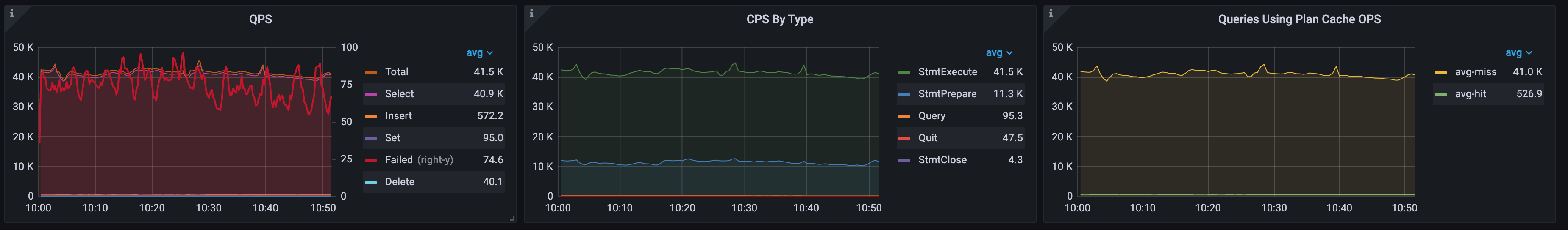
- In the QPS panel, the red bold line indicates the number of failed queries, and the Y axis on the right indicates the coordinate value of the number. In this example, the number of failed quries per second is 74.6.
- In the CPS By Type panel, the number of
StmtPreparecommands per second is much greater than that ofStmtCloseper second, which indicates that an object leak occurs in the application for prepared statements. - In the Queries Using Plan Cache OPS panel,
avg-missis almost equal toStmtExecutein the CPS By Type panel, which indicates that almost all SQL executions miss the execution plan cache.
KV/TSO Request OPS and KV Request Time By Source
- In the KV/TSO Request OPS panel, you can view the statistics of KV and TSO requests per second. Among the statistics,
kv request totalrepresents the sum of all requests from TiDB to TiKV. By observing the types of requests from TiDB to PD and TiKV, you can get an idea of the workload profile within the cluster. - In the KV Request Time By Source panel, you can view the time ratio of each KV request type and all request sources.
- kv request total time: The total time of processing KV and TiFlash requests per second.
- Each KV request and the corresponding request source form a stacked bar chart, in which
externalidentifies normal business requests andinternalidentifies internal activity requests (such as DDL and auto analyze requests).
Example 1: Busy workload
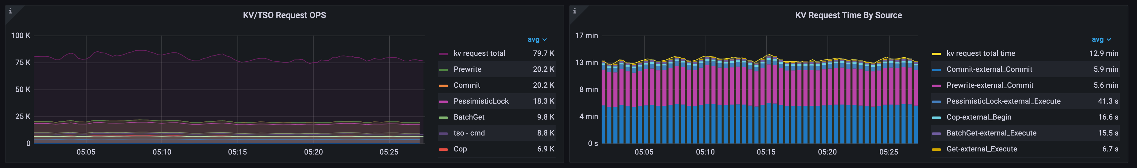
In this TPC-C workload:
- The total number of KV requests per second is 79,700. The top request types are
Prewrite,Commit,PessimisticsLock, andBatchGetin order of number of requests. - Most of the KV processing time is spent on
Commit-external_CommitandPrewrite-external_Commit, which indicates that the most time-consuming KV requests areCommitandPrewritefrom external commit statements.
Example 2: Analyze workload
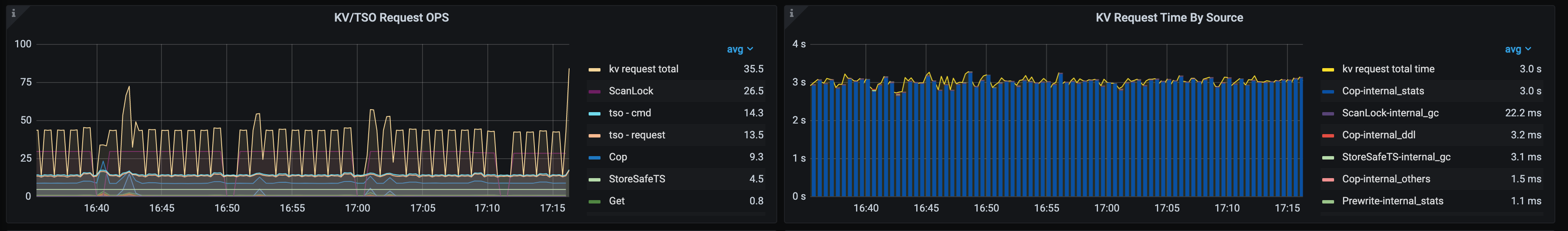
In this workload, only ANALYZE statements are running in the cluster:
- The total number of KV requests per second is 35.5 and the number of Cop requests per second is 9.3.
- Most of the KV processing time is spent on
Cop-internal_stats, which indicates that the most time-consuming KV request isCopfrom internalANALYZEoperations.
TiDB CPU, TiKV CPU, and IO usage
In the TiDB CPU and TiKV CPU/IO MBps panels, you can observe the logical CPU usage and IO throughput of TiDB and TiKV, including average, maximum, and delta (maximum CPU usage minus minimum CPU usage), based on which you can determine the overall CPU usage of TiDB and TiKV.
- Based on the
deltavalue, you can determine if CPU usage in TiDB is unbalanced (usually accompanied by unbalanced application connections) and if there are read/write hot spots among the cluster. - With an overview of TiDB and TiKV resource usage, you can quickly determine if there are resource bottlenecks in your cluster and whether TiKV or TiDB needs scale-out.
Example 1: High TiDB resource usage
In this workload, each TiDB and TiKV is configured with 8 CPUs.

- The average, maximum, and delta CPU usage of TiDB are 575%, 643%, and 136%, respectively.
- The average, maximum, and delta CPU usage of TiKV are 146%, 215%, and 118%, respectively. The average, maximum, and delta I/O throughput of TiKV are 9.06 MB/s, 19.7 MB/s, and 17.1 MB/s, respectively.
Obviously, TiDB consumes more CPU, which is near the bottleneck threshold of 8 CPUs. It is recommended that you scale out the TiDB.
Example 2: High TiKV resource usage
In the TPC-C workload below, each TiDB and TiKV is configured with 16 CPUs.

- The average, maximum, and delta CPU usage of TiDB are 883%, 962%, and 153%, respectively.
- The average, maximum, and delta CPU usage of TiKV are 1288%, 1360%, and 126%, respectively. The average, maximum, and delta I/O throughput of TiKV are 130 MB/s, 153 MB/s, and 53.7 MB/s, respectively.
Obviously, TiKV consumes more CPU, which is expected because TPC-C is a write-heavy scenario. It is recommended that you scale out the TiKV to improve performance.
Query latency breakdown and key latency metrics
The latency panel provides average values and 99th percentile. The average values help identify the overall bottleneck, while the 99th or 999th percentile or 999th helps determine whether there is a significant latency jitter.
Duration, Connection Idle Duration, and Connection Count
The Duration panel contains the average and P99 latency of all statements, and the average latency of each SQL type. The Connection Idle Duration panel contains the average and the P99 connection idle duration. Connection idle duration includes the following two states:
- in-txn: The interval between processing the previous SQL and receiving the next SQL statement when the connection is within a transaction.
- not-in-txn: The interval between processing the previous SQL and receiving the next SQL statement when the connection is not within a transaction.
An applications perform transactions with the same database connction. By comparing the average query latency with the connection idle duration, you can determine if TiDB is the bottleneck for overall system, or if user response time jitter is caused by TiDB.
- If the application workload is not read-only and contains transactions, by comparing the average query latency with
avg-in-txn, you can determine the proportion in processing transactions inside and outside the database, and identify the bottleneck in user response time. - If the application workload is read-only or autocommit mode is on, you can compare the average query latency with
avg-not-in-txn.
In real customer scenarios, it is not rare that the bottleneck is outside the database, for example:
- The client server configuration is too low and the CPU resources are exhausted.
- HAProxy is used as a TiDB cluster proxy, and the HAProxy CPU resource is exhausted.
- HAProxy is used as a TiDB cluster proxy, and the network bandwidth of the HAProxy server is used up under high workload.
- The network latency from the application server to the database is high. For example, the network latency is high because in public-cloud deployments the applications and the TiDB cluster are not in the same region, or the dns workload balancer and the TiDB cluster are not in the same region.
- The bottleneck is in client applications. The application server's CPU cores and Numa resources cannot be fully utilized. For example, only one JVM is used to establish thousands of JDBC connections to TiDB.
In the Connection Count panel, you can check the total number of connections and also the number of connections on each TiDB node, which helps you determine whether the total number of connections is normal and whether the number of connections on each TiDB node is unbalanced. active connections indicates the number of active connections, which is equal to the database time per second. The Y axis on the right (disconnection/s) indicates the number of disconnections per second in a cluster, which can be used to determine whether the application uses short connections.
Example 1: The number of disconnection/s is too high
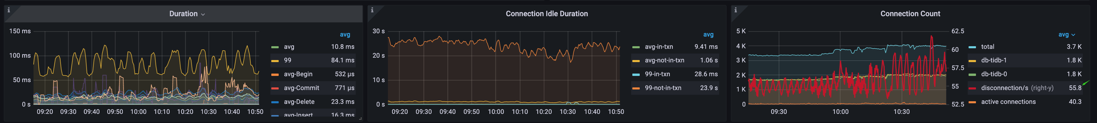
In this workload:
- The average latency and P99 latency of all SQL statements are 10.8 ms and 84.1 ms, respectively.
- The average connection idle time in transactions
avg-in-txnis 9.4 ms. - The total number of connections to the cluster is 3,700, and the number of connections to each TiDB node is 1,800. The average number of active connections is 40.3, which indicates that most of the connections are idle. The average number of
disonnnection/sis 55.8, which indicates that the application is connecting and disconnecting frequently. The behavior of short connections will have a certain impact on TiDB resources and response time.
Example 2: TiDB is the bottleneck of user response time

In this TPC-C workload:
- The average latency and P99 latency of all SQL statements are 477 us and 3.13 ms, respectively. The average latencies of the commit statement, insert statement, and query statement are 2.02 ms, 609 us, and 468 us, respectively.
- The average connection idle time in transactions
avg-in-txnis 171 us.
The average query latency is significantly greater than avg-in-txn, which means the main bottleneck in transactions is inside the database.
Example 3: TiDB is not the bottleneck of user response time

In this workload, the average query latency is 1.69 ms and avg-in-txn is 18 ms, indicating that TiDB spends 1.69 ms on average to process a SQL statement in transactions, and then needs to wait for 18 ms to receive the next statement.
The average query latency is significantly lower than avg-in-txn. The bottleneck of user response time is not in TiDB. This example is in a public cloud environment, where high network latency between the application and the database results in extremely high connection idle time, because the application and the database are not in the same region.
Parse, Compile, and Execute Duration
In TiDB, there is a typical processing flow from sending query statements to returning results.
SQL processing in TiDB consists of four phases, get token, parse, compile, and execute.
get token: Usually only a few microseconds and can be ignored. The token is limited only when the number of connections to a single TiDB instance reaches the token-limit limit.parse: The query statements are parsed into abstract syntax tree (AST).compile: Execution plans are compiled based on the AST from theparsephase and statistics. Thecompilephase contains logical optimization and physical optimization. Logical optimization optimizes query plans by rules, such as column pruning based on relational algebra. Physical optimization estimates the cost of the execution plans by statistics by a cost-based optimizer and selects a physical execution plan with the lowest cost.execute: The time consumption to execute a SQL statement. TiDB first waits for the globally unique timestamp TSO. Then the executor constructs the TiKV API request based on the Key range of the operator in the execution plan and distributes it to TiKV.executetime includes the TSO wait time, the KV request time, and the time spent by TiDB executor in processing data.
If an application uses the query or StmtExecute MySQL command interface only, you can use the following formula to identify the bottleneck in average latency.
avg Query Duration = avg Get Token + avg Parse Duration + avg Compile Duration + avg Execute Duration
Usually, the execute phase accounts for the most of the query latency. However, the parse and compile phases can also take a large part in the following cases:
- Long latency in the
parsephase: For example, when thequerystatement is long, much CPU will be consumed to parse the SQL text. - Long latency in the
compilephase: If the prepared plan cache is not hit, TiDB needs to compile an execution plan for every SQL execution. The latency in thecompilephase can be several or tens of milliseconds or even higher. If prepared plan cache is not hit, logical and physical optimization are done in thecompilephase, which consumes a lot of CPU and memory, makes Go Runtime (TiDB is written inGo) under pressure, and affects the performance of other TiDB components. Prepared plan cache is important for efficient processing of OLTP workload in TiDB.
Example 1: Database bottleneck in the compile phase

In the preceding figure, the average time of the parse, compile, and execute phases are 17.1 us, 729 us, and 681 us, respectively. The compile latency is high because the application uses the query command interface and cannot use prepared plan cache.
Example 2: Database bottleneck in the execute phase

In this TPC-C workload, the average time of parse, compile and execute phases are 7.39 us, 38.1 us, and 12.8 ms, respectively. The execute phase is the bottleneck of the query latency.
KV and TSO Request Duration
TiDB interacts with PD and TiKV in the execute phase. As shown in the following figure, when processing SQL request, TiDB requests TSOs before entering the parse and compile phases. The PD Client does not block the caller, but returns a TSFuture and asynchronously sends and receives the TSO requests in the background. Once the PD client finishes handling the TSO requests, it returns TSFuture. The holder of the TSFuture needs to call the Wait method to get the final TSOs. After TiDB finishes the parse and compile phases, it enters the execute phase, where two situations might occur:
- If the TSO request has completed, the Wait method immediately returns an available TSO or an error
- If the TSO request has not yet completed, the Wait method is blocked until a TSO is available or an error appears (the gRPC request has been sent but no result is returned, and the network latency is high)
The TSO wait time is recorded as TSO WAIT and the network time of the TSO request is recorded as TSO RPC. After the TSO wait is complete, TiDB executor usually sends read or write requests to TiKV.
- Common KV read requests:
Get,BatchGet, andCop - Common KV write requests:
PessimisticLock,PrewriteandCommitfor two-phase commits

The indicators in this section correspond to the following three panels.
- Avg TiDB KV Request Duration: The average latency of KV requests measured by TiDB
- Avg TiKV GRPC Duration: The average latency in processing gPRC messages in TiKV
- PD TSO Wait/RPC Duration: TiDB executor TSO wait time and network latency for TSO requests (RPC)
The relationship between Avg TiDB KV Request Duration and Avg TiKV GRPC Duration is as follows:
Avg TiDB KV Request Duration = Avg TiKV GRPC Duration + Network latency between TiDB and TiKV + TiKV gRPC processing time + TiDB gRPC processing time and scheduling latency
The difference between Avg TiDB KV Request Duration and Avg TiKV GRPC Duration is closely related to the network traffic, network latency, and resource usage by TiDB and TiKV.
- In the same data center: The difference is generally less than 2 ms.
- In different availability zones in the same region: The difference is generally less than 5 ms.
Example 1: Low workload of clusters deployed on the same data center

In this workload, the average Prewrite latency on TiDB is 925 us, and the average kv_prewrite processing latency inside TiKV is 720 us. The difference is about 200 us, which is normal in the same data center. The average TSO wait latency is 206 us, and the RPC time is 144 us.
Example 2: Normal workload on public cloud clusters

In this example, TiDB clusters are deployed in different data centers in the same region. The average commit latency on TiDB is 12.7 ms, and the average kv_commit processing latency inside TiKV is 10.2 ms, a difference of about 2.5 ms. The average TSO wait latency is 3.12 ms, and the RPC time is 693 us.
Example 3: Resource overloaded on public cloud clusters

In this example, the TiDB clusters are deployed in different data centers in the same region, and TiDB network and CPU resources are severely overloaded. The average BatchGet latency on TiDB is 38.6 ms, and the average kv_batch_get processing latency inside TiKV is 6.15 ms. The difference is more than 32 ms, which is much higher than the normal value. The average TSO wait latency is 9.45 ms and the RPC time is 14.3 ms.
Storage Async Write Duration, Store Duration, and Apply Duration
TiKV processes a write request in the following procedure:
scheduler workerprocesses the write request, performs a transaction consistency check, and converts the write request into a key-value pair to be sent to theraftstoremodule.The TiKV consensus module
raftstoreapplies the Raft consensus algorithm to make the storage layer (composed of multiple TiKVs) fault-tolerant.Raftstore consists of a
Storethread and anApplythread:- The
Storethread processes Raft messages and newproposals. When a newproposalsis received, theStorethread of the leader node writes to the local Raft DB and copies the message to multiple follower nodes. When thisproposalsis successfully persisted in most instances, theproposalsis successfully committed. - The
Applythread writes the committedproposalsto the KV DB. When the content is successfully written to the KV DB, theApplythread notifies externally that the write request has completed.
- The

The Storage Async Write Duration metric records the latency after a write request enters raftstore. The data is collected on a basis of per request.
The Storage Async Write Duration metric contains two parts, Store Duration and Apply Duration. You can use the following formula to determine whether the bottleneck for write requests is in the Store or Apply step.
avg Storage Async Write Duration = avg Store Duration + avg Apply Duration
Example 1: Comparison of the same OLTP workload in v5.3.0 and v5.4.0
According to the preceding formula, the QPS of a write-heavy OLTP workload in v5.4.0 is 14% higher than that in v5.3.0:
- v5.3.0: 24.4 ms ~= 17.7 ms + 6.59 ms
- v5.4.0: 21.4 ms ~= 14.0 ms + 7.33 ms
In v5.4.0, the gPRC module has been optimized to accelerate Raft log replication, which reduces Store Duration compared with v5.3.0.
v5.3.0:

v5.4.0:

Example 2: Store Duration is a bottleneck
Apply the preceding formula: 10.1 ms ~= 9.81 ms + 0.304 ms. The result indicates that the latency bottleneck for write requests is in Store Duration.

Commit Log Duration, Append Log Duration, and Apply Log Duration
Commit Log Duration, Append Log Duration, and Apply Log Duration are latency metrics for key operations within raftstore. These latencies are captured at the batch operation level, with each operation combining multiple write requests. Therefore, the latencies do not directly correspond to the Store Duration and Apply Duration mentioned above.
Commit Log DurationandAppend Log Durationrecord time of operations performed in theStorethread.Commit Log Durationincludes the time of copying Raft logs to other TiKV nodes (to ensure raft-log persistence).Commit Log Durationusually contains twoAppend Log Durationoperations, one for the leader and the other for the follower.Commit Log Durationis usually significantly higher thanAppend Log Duration, because the former includes the time of copying Raft logs to other TiKV nodes through network.Apply Log Durationrecords the latency ofapplyRaft logs by theApplythread.
Common scenarios where Commit Log Duration is long:
- There is a bottleneck in TiKV CPU resources and the scheduling latency is high
raftstore.store-pool-sizeis either excessively small or large (an excessively large value might also cause performance degradation)- The I/O latency is high, resulting in high
Append Log Durationlatency - The network latency between TiKV nodes is high
- The number of the gRPC threads are too small, CPU usage is uneven among the GRPC threads.
Common scenarios where Apply Log Duration is long:
- There is a bottleneck in TiKV CPU resources and the scheduling latency is high
raftstore.apply-pool-sizeis either excessively small or large (an excessively large value might also cause performance degradation)- The I/O latency is high
Example 1: Comparison of the same OLTP workload in v5.3.0 and v5.4.0
The QPS of a write-heavy OLTP workload in v5.4.0 is improved by 14% compared with that in v5.3.0. The following table compares the three key latencies.
In v5.4.0, the gPRC module has been optimized to accelerate Raft log replication, which reduces Commit Log Duration and Store Duration compared with v5.3.0.
v5.3.0:

v5.4.0:

Example 2: Commit Log Duration is a bottleneck

- Average
Append Log Duration= 4.38 ms - Average
Commit Log Duration= 7.92 ms - Average
Apply Log Duration= 172 us
For the Store thread, Commit Log Duration is obviously higher than Apply Log Duration. Meanwhile, Append Log Duration is significantly higher than Apply Log Duration, indicating that the Store thread might suffer from bottlenecks in both CPU and I/O. Possible ways to reduce Commit Log Duration and Append Log Duration are as follows:
- If TiKV CPU resources are sufficient, consider adding
Storethreads by increasing the value ofraftstore.store-pool-size. - If TiDB is v5.4.0 or later, consider enabling
Raft Engineby settingraft-engine.enable: true. Raft Engine has a light execution path. This helps reduce I/O writes and long-tail latency of writes in some scenarios. - If TiKV CPU resources are sufficient and TiDB is v5.3.0 or later, consider enabling
StoreWriterby settingraftstore.store-io-pool-size: 1.
If my TiDB version is earlier than v6.1.0, what should I do to use the Performance Overview dashboard?
Starting from v6.1.0, Grafana has a built-in Performance Overview dashboard by default. This dashboard is compatible with TiDB v4.x and v5.x versions. If your TiDB is earlier than v6.1.0, you need to manually import performance_overview.json, as shown in the following figure:
